8 Differential Equations

8.1 Ordinary Differential Equations

Perhaps the most important differential equation is the exponential growth (or decay) equation. The derivative of \(y(t)=\mbox{e}^{rt}\) is \(\mbox{d}y(t)/\mbox{d}t=r\mbox{e}^{rt}\), which means \[\begin{equation} \frac{\mbox{d}y(t)}{\mbox{d}t}=r y(t). \tag{8.1} \end{equation}\] The equation says that the rate of change in \(y\) depends on the value of \(y\) itself. When \(y\) grows, the slope \(\mbox{d}y/\mbox{d}t\) becomes steeper. When \(t\rightarrow\infty\), the function \(\mbox{e}^{rt}\) grows exponentially if \(r>0\), while the function \(\mbox{e}^{rt}\) decays exponentially if \(r<0\).

Thomas Malthus depicted a situation where equation (8.1) can describe the growth of the population (for \(r>0\)). Malthus (1798) proposed two laws on mankind’s nature,

• Malthus’ law 1: Food is necessary to the existence of man.

• Malthus’ law 2: The passion between the sexes is necessary and will remain nearly in its present state.

These two laws can represent two forces of the growth, production growth in the earth from Malthus’ law 1 and population growth from Malthus’ law 2. The second law, as shown in the (oversimplified) example of Fibonacci’s rabbits in chapter 4.3, will deduce an exponential growth of population. Malthus suspects the earth has the power to produce such an exponential growth for subsisting the population. In other words, if we consider the population size as an exponential growth process, the production from the earth in Malthus’ sense can not grow as fast as an exponential growth process. This fundamental difference between the two growth patterns will eventually cause inequality. Malthus argues that man cannot escape from such a natural inequality of these two powers. This inequality is known as the Malthusian trap, where the excessive population would outstrip their resources104104 Malthus (1798) proposed a question at the beginning, “whether man shall henceforth start forwards with accelerated velocity towards illimitable, and hitherto unconceived improvement, or be condemned to a perpetual oscillation between happiness and misery, and after every effort remain still at an immeasurable distance from the wished-for goal.” The latter situation could be the expected consequence of Malthusian trap.

For the Malthusian population growth model, \(y\) stands for the size of the population. The size \(y(\cdot)\) is a function depending on time \(t\), and the growth rate \(r\) is the parameter of this model. So the equation \(\mbox{d}y/\mbox{d}t=ry\) tells that at time \(t\), the rate of the instantaneous population change \(\mbox{d}y/\mbox{d}t\) equals the instantaneous growing population, namely the growth rate \(r\) times the total population \(y(t)\).

Equation (8.1) has been applied in many different fields. For example, the inflation model or the interest rate model in economics and finance can be cast in this form. In this case, we consider \(y\) as the price and \(\mbox{d}y/\mbox{d}t\) as the instantaneous price change. The equation tells that \(\mbox{d}y/\mbox{d}t\) equals the (fixed) interest rate \(r\) times the current price \(y(t)\).

Recall that the exponential growth \(e^{x}\) increases more rapidly than the polynomial growth \(x^{N}\) no matter what \(N\in\mathbb{N}\) is.105105 Taylor series of \(e^{x}\) gives \(e^{x}=\sum_{n=0}^{\infty}x^n/(n!)\). Thus \[\lim_{x\rightarrow\infty}\mbox{e}^{x}/x^{N}\approx \lim_{x\rightarrow\infty}\sum_{n=N}^{\infty}x^n/(n!)=\infty.\] That is, \(\lim_{x\rightarrow\infty}\mbox{e}^{x}/x^{N}=\infty\) for any value of \(N\). So \(\mbox{e}^{x}\) must grow faster than \(x^{N}\) for any \(N\in\mathbb{N}\). Given some fixed value \(N\), we expect that \(e^{x}>x^{N}\) for a large enough \(x\). That means the exponential growth effect is more significant when the base is large. From figure 8.1 and 8.2, we can see the most two populous countries, China and India, have more significant population expansions than the others. Without the industrial revolutions and technological innovations, in a Malthusian trap, the production would be either a polynomial growth process or a certain fixed amount of resources in the limit.

The following data table (data source: https://www.gapminder.org/data/) gives an overview about the world population and GDP per capita from 1952 to 2007. We can see that Malthusian trap hasn’t happened so far in a wide range. However, if we analyze some figures, i.e. those of Afghanistan, we can indeed find the shadows of the trap.

Figure 8.1: Top 10 Populous Countries (1952-2007)

Figure 8.2: World Population (1952-2007)

The differential equation (8.1) is an autonomous equation because \(\mbox{d}y/\mbox{d}t\) only depends on the value of itself.106106 When there is another time-dependent variable in the equation, such as \(\mbox{d}y/\mbox{d}t=ry+\cos t\), then the equation is nonautonomous. Fundamental to the study of differential equations is to solve the equation. It means that we need to find a function that explicitly specifies a rule to determine the values of \(y(t)\). For example, if we only look at equation (8.1), it is not immediately clear why the equation models exponential growth. However, this becomes quite evident with an examination of the solution \(y(t)=\mbox{e}^{rt}\) to this problem.

The solution to a differential equation must be a function of time, as the differentiation is with respect to time. It may be interesting to see that \(\mbox{e}^{rt}\) is not the only solution for equation (8.1). If we set \(y(t)=\mbox{e}^{rt+1}=\mbox{e}^{rt}\mbox{e}\), we will find that it also satisfies the equation. In fact, for any constant \(C\), the solution \(\mbox{e}^{rt+C}\) will work. To see this, we rewrite the expression as \(\mbox{d}y/y=r\mbox{d}t\), and have the solution \(\ln y=rt+C\), or say \(y(t)=\mbox{e}^{rt}\mbox{e}^{C}\). Notice that \[\frac{\mbox{d}\mbox{e}^{rt}\mbox{e}^{C}}{\mbox{d}t}=\mbox{e}^{C}\frac{\mbox{d}\mbox{e}^{rt}}{\mbox{d}t}=r\mbox{e}^{rt}\mbox{e}^{C}\Leftrightarrow\frac{\mbox{d}y(t)}{\mbox{d}t}=r\times y(t).\] In order to achieve a unique solution, we need a condition to fix the value \(C\). Suppose we know a starting value \(y_{0}\) at \(t=0\), then the solution function \(y(0)=\mbox{e}^{r\times0}\mbox{e}^{C}=\mbox{e}^{C}\) tells that \(y_{0}=\mbox{e}^{C}\) or \(C=\ln y_{0}\). Such a condition is called the initial condition. Thus we rewrite equation (8.1) as \[\frac{\mbox{d}y(t)}{\mbox{d}t}=ry(t),\;\mbox{with }y(0)=y_{0}\mbox{ at }t=0\] so that it has a unique solution \(y(t)=y_{0}\mbox{e}^{rt}\). This solution \(y_{0}\mbox{e}^{rt}\) is called the general solution of equation (8.1), while \(\mbox{e}^{rt}\) is called a particular solution for the case \(y_{0}=1\). The problem of determining a unique solution to the differential equation with initials is called the initial value problem.

The exponential growth is a monotonic phenomenon. Based on his laws of mankind’s nature, Malthus also predicted a tendency that human numbers would stop growing due to the shortage of food supply. Under the excessed population and the insufficient provision ( Malthusian trap), the society would have been threatened by unstable factors in the form of poverty, disease, starvation, or any event or circumstance that could shorten the human life span (war, plague and famine, poor health and economic conditions). Therefore, Malthus argued to arrange the social system by keeping the two unequal powers of growth equal. In his view, checks (slow down the progress) in the form of birth, marriage, and some other social factors are necessary to keep societies from moving beyond their means of subsistence.107107 “Yet in all societies, even those that are most vicious, the tendency to a virtuous attachment is so strong that there is a constant effort towards an increase of population. This constant effort as constantly tends to subject the lower classes of the society to distress and to prevent any great permanent amelioration of their condition” - Malthus (1798) Malthus’s simple but powerful proposition “That population cannot increase without the means of subsistence” may be controversial in his time; however, today, his name has become a byword for active concern about humankind’s demographic and ecological prospects.

We can model the above tendency by differential equations. Consider that the population growth rate consists of two constant terms, the birth rate \(b\) and the death rate \(d\). The net rate of the growth is \(r=b-d\). Now the model of population growth becomes \[\begin{equation} \frac{\mbox{d}y}{\mbox{d}t}=by-dy=ry. \tag{8.2} \end{equation}\] Equation (8.2) is known as the birth-death equation (or inflow-outflow equation). It is one of the most straightforward ways to express the changes in a dynamical system. For example, in a system of stocks and flows, the equation expresses the system’s stocks one by one, and record the inflow and outflow of each stock. For a bank account, the inflows are deposits and interest, and the outflows are withdrawals. For an animal population, the inflows are birth and immigration (migration into the population), while the outflows are death and emigration (migration out of the population).108108 When the inflow energies and the outflow energies are equivalent, the system is conservative.

For the population of community, the birth-death equation can model the effect of checking. The inflows, say \(r_{1}y\), model the exponential growth caused by “the passion between the sexes.” Then the outflows model a tendency of surpressing the exponential growth effect. One can consider \(r_{2}y^{2}\) as the outflows, since the qaudratic \(-y^{2}\) can surpress the linear \(y\) when the population \(y\) becomes large. In reality, such a tendency could happen either intentionally, such as Chinese demographic policy, and the increase of legal marriage age in most countries (delay marriage), or obliviously, such as the awakens of feminism, and the demand of enhancing health and economic conditions among the middle class.109109 “…whatever has existed to early marriages, among the lower classes, from a fear of not providing well for their families, or among the higher classes, from a fear of lowering their condition in life. Consequently in no state that we have yet known has the power of population been left to exert itself with perfect freedom.” (1798)

To combine these two effects, we have the following birth-death equation \[\begin{equation} \frac{\mbox{d}y}{\mbox{d}t}=r_{1}y-r_{2}y^{2}=r_{1}y\left(1-\frac{r_{2}}{r_{1}}y\right), \tag{8.3} \end{equation}\] which is called the logistic differential equation. When \(1-\frac{r_{2}}{r_{1}}y(t)=0\), \(\mbox{d}y/\mbox{d}t\) in equation (8.3) becomes zero. The zero growth means that an equilibrium point (also called steady state or stationary point) appears. That is, if the population of the community \(y(t)\) in (8.3) equals the ratio \(r_{1}/r_{2}\), the community reaches its equilibrium popluation size. Thus, \(r_{1}/r_{2}\) represents the carrying capacity of the community.110110 We can verify that the logistic function \(y(t)=1/(1+\mbox{e}^{-t})=\mbox{e}^{t}/(1+\mbox{e}^{t})\) is the solution of the differential equation (8.3) when \(r_{1}=r_{2}=1\). \[\frac{\mbox{d}y}{\mbox{d}t}=\frac{\mbox{e}^{t}}{(1+\mbox{e}^{t})^{2}}= \\ \frac{\mbox{e}^{t}}{(1+\mbox{e}^{t})}\frac{1}{(1+\mbox{e}^{t})}=y(t)(1-y(t)).\] When \(t\rightarrow\infty\), \(y(t)\) converges to \(\lim_{t\rightarrow\infty}y(t)=1/(1+\mbox{e}^{t})=1\) that equals \(r_{1}/r_{2}=1\). If we know the initial condition \(y(0)=C\), then the general solution becomes \(y(t)=C/(1+\mbox{e}^{-t})\). The solution of (8.3) is \[y(t)=\frac{r_{1}}{r_{2}}\left(1+\frac{r_{1}/r_{2}-y(0)}{y(0)}\mbox{e}^{-r_{1}t}\right)^{-1}\] with \(\lim_{t\rightarrow\infty}y(t)=r_{1}/r_{2}\). When \(t\) goes to infinity, the solution of this logistic model converges to this carrying capacity \(r_{1}/r_{2}\), namely \(\lim_{t\rightarrow\infty}y(t)=y^{*}=r_{1}/r_{2}\). We call the limit \(y^{*}\) the steady state of the differential equation. In this logistic model, the increase of population is limited by the size and fertility of the community, with the result that the population gets ever-closer to a steady state value \(r_{1}/r_{2}\). The logistic curve begins with rapid growth characteristic of the birth rate (positive feedback from the system), followed by slower growth that is dominated by the death rate (negative feedback from the system). Figure 8.3 illustrates this trend. The equation converges to the carrying capacity independently of the initial value.

8.2 Numerical Example: Euler’s Scheme

The analytical form of the solution of logistic growth models is more difficult to derive than the exponential growth models. In fact, most differential equation models may not have analytic solutions. This is a common issue for differential equations. As the models get more complicated, the challenge of finding an analytic solution to the models becomes more serious. Very often the challenge becomes impossible to overcome. It is for this reason that the numerical methods are frequently used for solving differential equation models rather than were the analytical derivations.

The general formulation of autonomous differential equation problem with a given initial condition is given as follows \[\begin{equation} \frac{\mbox{d}y}{\mbox{d}t}=f(y),\quad y(0)=c \tag{8.4} \end{equation}\] where \(f(\cdot)\) is a Lipschitz continuous function of the state variable \(y(t)\). The equilibrium point (steady state or stationary point) is denoted by \(y^{*}\). If the model converges to the equilibrium point, we expect that \(\lim_{t\rightarrow\infty}y(t)=y^{*}\), namely \(\lim_{t\rightarrow\infty}f(y(t))=f(y^{*})=0\). The equilibrium point may not exist for many differential equations. For example, the exponential growth model has a monotone increasing feature such that \(y(t)\) goes to infinity as \(t\rightarrow\infty\). There is no equilibrium in such a monotone growth.

A basic numerical method of solving the problem in (8.4) is the Euler’s scheme. The idea of this method is to discretize a continuous time curve into a series of the slopes at different time points of the curve. For \(dy/dt=f(y)\), the slope of \(y(t)\) at time \(t_{0}\) is \(f(y(t_{0}))\). We can collect a series of slopes, \(f(y(t_{0})),\dots,f(y(t_{N+1}))\), at time \(t_{1},\dots,t_{N+1}\). Suppose these points have an equal step size \(h\), such that \(t_{n+1}=t_{n}+h\) for \(n=1,\dots,N\). Then the differentiation \(dy/dt\) can be descritized into \[f(t,y)=\frac{\mbox{d}y}{\mbox{d}t}\approx\frac{y(t+h)-y(t)}{h}.\] We have an iterative representation: \(y(t+h)=y(t)+hf(y(t))\). In other words, \(y(t_{n+1})=y(t_{n})+hf(y(t_{n}))\) for \(n=1,\dots,N-1\). Given the initial condition \(y(0)=y(t_{0})\), the iteration gives \(y(t_{1}), y(t_{2}),\dots,y(t_{N+1})\) recursively. The value of the series \((y(t_{n}))_{n=1}^{N+1}\) is the approximation of the solution to the differential equation in (8.4).

The following code implements this scheme on the logistic differential equation (8.3) with \(r_1=r_2=1\) and \(y^*=1\).

y = time = 1:100;  t0 = 0; y0 = 0.1; h = 0.1; 
y[1] = y0; time[1]=t0; 

for(n in c(1:99)){
    y[n+1] = y[n] + h * y[n]  * (1 - y[n])
    time[n+1] = time[n] + h
}

# Plot the equation
dat = data.frame(time,y)
library(ggplot2); library(gganimate)
fig = ggplot(dat, aes(x=time, y=y)) 
fig + geom_point(color="blue") +  transition_time(time=time) + shadow_mark() + geom_hline(aes(yintercept=1),color="red",alpha=0.5) + theme_minimal()

For the root-finding problems \(f(y^{*})=0\), seeking the root \(y^{*}\) by the fixed point iteration relates to the Euler’s scheme for computing an equilibrium. That is, the root \(y^{*}\) can be found by running a differential equation \(\mbox{d}y/\mbox{d}t=f(y)\). By the definition of the equilibrium \(y^{*}\), we know that the steady \(y^{*}\) gives both the zero derivative in \(\mbox{d}y/\mbox{d}t|_{y=y^{*}}=0\) and the root of \(f(\cdot)\). If the function \(f(y)\) can be constructed by a fixed point iteration \(g(y)=y\) such that \(f(y)=h^{-1}(g(y)-y)\), with the non-zero constant (step size) \(h\), then one has \(f(y^{*})=0\) if and only if \(g(y^{*})=y^{*}\). So the convergence problem of \(\mbox{d}y/\mbox{d}t=f(y)=0\) is equivalent to the problem of finding fixed points of the function\[\frac{\mbox{d}y}{\mbox{d}t}=f(y^{*})=0\Leftrightarrow g(y^{*})=y^{*}.\] The Euler’s scheme can be derived from the fixed point iteration \[f(y_{t+1})=\frac{g(y_{t})-y_{t}}{h}=\frac{y_{t+1}-y_{t}}{h}.\] Therefore, the equilibrium point is also named as the fixed point for the iteration \(y_{t+1}=g(y_{t})\). We will come back to this discussion in section 8.4.

8.3 Miscellaneous: Mechanistic Worldview

When we look back to equation (8.1) and its solution, we may come up with an interesting view: the growth or the decay described by the equation is determined. With an appropriate initial condition, one can predict the future or “retrodict” the past with certainty. That is, by calculating the solution \(y_{0}\mbox{e}^{rt}\) of the differential equation, we can govern the state information \(y(T)\) at time \(T\), the subsequent states \((y(t))_{t>T}\), as well as the preceding states \((y(t))_{t<T}\). The solution \(y(\cdot)\) becomes a “law,” with which we explain or interpret past events and also infer the future ones. In the model of differential equations, there is no mathematical distinction between the past and the future. All the information regarding the dynamics of the system is embodied in \(y(t)\). By modifying the value of \(t\), we can come up with different \(y(t)\) that represents the different information at different \(t\).

The law can be thought of as the first cause in Aristotle’s metaphysics, where Aristotle called it God. The first cause is the thing that originates motion, and that itself is unmoved, eternal, and actual. We can see the law \(y(\cdot)\) that initiates the movement at \(y_{0}\) is unmoved, eternal, and actual. Under this law, each event is “caused” by some preceding events, so that every event can be explained or predicted. Such a law now refers to mechanical law.

René Descartes, who is often considered as one of the founders of modern philosophy and is best known for his line “Cogito, ergo sum” (“I think, therefore I am”), sketched the outlines of a mechanistic approach to biology, physics, psychology, and medicine. Descartes’ method is analytic, known as Cartesian reductionism.111111 In their attempt to abandon European influences, the American artists created the abstract expressionism. This abstract art intends to show us the world by exploring the relationship of shapes, spaces, and colors to one another. The artists explore the nature of visual representation by reducing images to their essential elements of form, line, color, or light. The perception of a single line, a complex scene, or a work of art can evoke powerful feelings. A few expert brushstrokes can create a portrait of an individual that is far more compelling than a person in the flesh; a particular combination of colors can evoke a sense of serenity, anxiety, or exaltation. By reducing figuration, artists enable us to perceive an essential component of the work. It consists of breaking up thoughts and problems into pieces and arranging these in their logical order. The method suggests that all aspects of complex phenomena can be understood by reducing them to their smallest constituent parts.

The causes of motion in Descartes’ view were in terms of each motion being generated by contact with prior contiguous motion. Thus the material universe was a perfect machine, governed by exact mathematical laws. His separation of mind from matter is known as the Cartesian division. There was no purpose, life, or spirituality in the matter. Nature worked according to mechanical laws, and everything in the material world could be explained in terms of the movement of its parts. This mechanical picture of nature became the dominant paradigm of science in the 17th century.

Newton developed a comprehensive mathematical formulation of the mechanistic view of nature. He then used his new mathematical method to formulate the exact laws of motion for all bodies under the influence of the force and the gravity. The significance of these laws lays in their universal applications. Newton’s laws are invariant with respect to the time. Therefore, the past and future play the same role. These laws were found to be valid throughout the solar system and thus seemed to confirm the Cartesian view of nature. In such an order, once initial conditions are given, everything is determined. Thus the Newtonian universe is one huge mechanical system operating according to exact mathematical laws. Nature is an automaton, which humankind can control, at least in principle.112112 Perpetual oscillations between the world as an automaton and the theology in which God governs the universe is a duality that has plagued Western thought ever since. But in fact, both sides of this duality are forms of determinism. The initial state, in the Newtonian view, was given by God. God created the material particles, the forces between them, and the fundamental laws of motion. In this way, the whole universe was set in motion, and it has continued to run ever since, like a machine, governed by immutable laws. The mechanistic view of nature is thus closely related to a rigorous determinism, with the giant cosmic machine completely causal and determinate. The whole universe looked like a clockwork. What could be the meaning of human freedom in a deterministic world of atoms? The answer cannot be found in the deterministic framework.

Newtonian mechanics was extended far beyond the description of the natural and physical phenomena. Apart from the demography, mechanical laws also became the cornerstone in economics and sociology. The calculus of prices and utilities is a counterpart of the differential calculus. Laissez-faire (free-market) from the French Physiocrats or invisible hand from Adam Smith reflects the belief on the existence of a natural rule in governing the economic affairs. Even on the opposite side of this market fundamentalism, the technological determinism (a belief on the technological development determining social changes), and historical materialism (a belief on a society’s productive forces and relations of production determining society’s organization and development) from Karl Marx relate to this mechanistic worldview. Nowadays, Newtonian mechanics had lost its role as the fundamental theory of natural phenomena since the emergence of quantum physics, electromagnetics, and other theories. Nevertheless, the basic ideas underlying Newtonian physics, though insufficient to explain all natural phenomena, are believed to be correct.

8.4 Example: Tâtonnement and Stability

Equilibrium is also a well-known concept for describing the behaviors of economic variables in a hypothetical laissez-faire (free-market or free-competition) environment. In the early 20th century, Léon Walras, a leading figure in the marginalist revolution in economics, proposed a law (or a market clear condition) saying that the sum of the demands and supplies across all commodities in an economy must equal zero. This law also claims that prices adjust in response to excess quantities (in terms of demands or supplies). That is, the price is adjusted through the interaction of supply and demand. When price increases, buyers from the demand side of the market pursue lower quantities while sellers from the supply side offer typically higher quantities. The actions will reverse when the price decreases. In this environment, both the sellers and buyers are price takers. Each side is willing to trade until the price reaches the steady or the equilibrium level. When the equilibrium exists, all commodity markets simultaneously satisfy Walras’ law. Thus the pricing mechanism in such a free market economy is self-adjusting. Under this mechanism, price equates supply and demand of each commodity to clear the market through which the economic equilibrium can be achieved. Walras suggested a process called tâtonnement, a presumably global convergent algorithm (a convergence with an arbitrary initial point), for modeling the above procedure of approaching an economic equilibrium.

To illustrate the tâtonnement mechanism, let’s consider an economy with only one commodity. The price of this commodity is a time-dependent state variable \(p(t)\). The market of this particular commodity is in equilibrium if the quantity of the demand \(d\) equals that of supply \(s\). In other words, the demand minus supply equals zero (\(d-s=0\)). Let’s assume that both the demand and the supply depend on the price so that they are functions of \(p\), denoted by the demand function \(d(p)\) and the supply function \(s(p)\), respectively. The Walras’ law is the condition \(f(p^{*})=d(p^{*})-s(p^{*})=0\) where \(p^{*}\) stands for the equilibrium price.113113 The function \(f(\cdot)\) is also called the excess demand function. The condition \(f(p^{*})=0\) can be extended to a market with \(N\in\mathbb{N}\) commodities. Then we have \(f(p^{*})=0\) if and only if \(d(p^{*})=s(p^{*})\), namely equating the demand and the supply.

Normally, the demand function \(d(p)\) is assumed to be negatively correlated to the price. That is, the lower the price is, the higher the demand (downward-sloping). The supply function \(s(p)\) is normally assumed to be the opposite, namely, the higher the price is, the higher the supply (upward-sloping).114114 The doctrine of marginalism is that the demand and supply are explained in terms of marginal quantities. In the views of marginalism, the demand function is constructed by the marginal rates of substitution. That is, at any given price, a prospective buyer has the marginal rate of substitution of money for the commodity. The rate represents the willingness to spend money on the commodity. It decreases as the buyer possesses more commodity or spends more money (called the law of diminishing marginal utility). Therefore, any buyer has a demand function that decreases in response to the price increase. The demand in the market is an aggregate quantity of all buyers’ demand. Similarly, the supply function is constructed by the marginal cost or the law of diminishing marginal productivity. The supply function can be thought of as complementary to the demand function. We can consider the linear demand and supply function as an example: \[d(p)=\beta_{0}+\beta_{1}p,\; s(p)=\alpha_{0}+\alpha_{1}p\] with the conditions \(\beta_{1}<0\) and \(\alpha_{1}>0\) that fit the requirements of being downward-sloping and upward-sloping (see the right part of figure 8.4).

Figure 8.4: Tâtonnement and supply-demand

The tâtonnement mechanism assumes that the instantaneous price change \(\mbox{d}p/\mbox{d}t\) depends on the difference between the demand and the supply (a birth death equation)such that \[\frac{\mbox{d}p}{\mbox{d}t}=f(p)=d(p)-s(p)=(\beta_{0}-\alpha_{0})+(\beta_{1}-\alpha_{1})p.\] At time \(t=0\), one can set an initial condition \(p(0)\) to the price. The tâtonnement mechanism describes the convergence of the market price \(p(t)\) to the equilibrium price \(p^{*}\) so that \(f(p^{*})=0\).115115 For the linear demand and supply function, we have the analytical form for the equilibrium price \(p^{*}=(\beta_{0}-\alpha_{0})/(\alpha_{1}-\beta_{1})\). The solution to this differential equation is \(p(t)=(p^{*}-p(0)\mbox{e}^{-(\beta_{1}-\alpha_{1})t}+p^{*}\) with \(\lim_{t\rightarrow\infty}f(p(t))=f(p^{*})=0\). The left part of figure 8.4 draws the solution \(p(t)\). In this example, the tâtonnement guides the price process converge to the equilibrium value regardless of the initial price \(p(0)\). Thus this tâtonnement obtains a global convergent feature. According to the tâtonnement process, the free market doctrine is equivalent to the belief of a global convergent mechanism for the market clear condition (Walras’ law) \(f(p)=d(p)-s(p)=0\) where no intervention or regulation is needed to guide the price converge to the equilibrium level \(p^{*}\) where \(f(p^{*})=0\).

It was believed that Walrasian tâtonnement was a global convergent mechanism, which means that any initial price will clear the market after a long enough period. Unfortunately, this globally convergent result fails for the general functional forms of demands and supplies. For example, if \(\beta_{1}-\alpha_{1}<0\) (both supply and demand have the same direction of the slopes, and supply slope is steeper), then the process will diverge as \(\lim_{t\rightarrow\infty}\mbox{e}^{-(\beta_{1}-\alpha_{1})t}\rightarrow\infty\). Moreover, for nonlinear \(d(\cdot)\) and \(s(\cdot)\), most likely, the convergences are local. That is, the tâtonnement process converges under some initials but does not under some others.

Figure 8.5: Divergence

There are many situations where the initial value matters. Consider the fixed point iteration in figure 3.1, the iteration converges with the initial point \(x_{0}=1.4\) in figure 3.1, but in figure 8.5, it diverges with \(y_{0}=1.55\). Thus, this is a local convergent example. The consequence of the local convergence affects the stability of the process. Stability tells whether an initial “error” will grow. Consider a convergent process given an initial \(y_{0}\). Suppose that we give some (infinitesimal) error \(\epsilon\) to the initial condition \(y_{0}+\epsilon\), after a long enough period, if the “error” does not grow, then the process is stable. We can capture the basic idea by the linear approximation (1st order Taylor series). Suppose \(y_{t+1}=g(y_{t})\), the difference \(y_{t+1}-y^{*}\) is the same as \(g(y_{t})-g(y^{*})\). Therefore, \[y_{t+1}-y^{*}=g(y_{t})-g(y^{*})\approx\left.\frac{\mbox{d}g}{\mbox{d}y}\right|_{y_{t}}(y_{t}-y^{*}).\] If \(|\mbox{d}g/\mbox{d}y|<1\) at \(y_{t}\), then \(y_{t}\) is attracted to the fixed point \(y^{*}\); if \(|\mbox{d}g/\mbox{d}y|>1\), \(y_{t}\) is repelled to \(y^{*}\). The previous problem in figure 3.1 and 8.5 has two fixed points. One is around \(0.6124\) and the other is around \(1.5423\). For \(0.6124\), \(|\mbox{d}g/\mbox{d}y|<1\) at the fixed point \(y^{*}=0.6124\), so \(0.6124\) is an attracting fixed point. For \(1.5423\), \(|\mbox{d}g/\mbox{d}y|>1\), so \(1.5423\) is a repelling fixed point. Thus although the initial \(1.4\) in figure 3.1 and \(1.55\) in figure 8.5 both are closed to \(1.5423\), one iteration (\(1.4<1.5423\)) is repelled to the fixed point \(0.6124\) and the other iteration (\(1.55>1.5423\)) is repelled to infinity.116116 Classical science emphasized order and stability; however, in reality, in contrast, we see fluctuations, instability, multiple choices, and limited predictability at all levels of observation. Soon we will confront a situation which William James called a dilemma of determinism. Is the future given, or is it under perpetual construction? These contradictory attitudes relate to our explanations of the meaning of time. See Ch [].

fixedpoint = function(ftn, y0, tol, max.iter) {
  yold = y0;
  ynew = ftn(yold)
  iter = 1;
  cat("At iteration 1 value of y is:", ynew, "\n")
  yold = ynew;
  ynew = ftn(yold);
  iter = iter + 1;
  for ( iter in 2:max.iter-1){
    if (abs(ynew-yold) > tol) {
      yold = ynew;
      ynew = ftn(yold);
      iter = iter + 1
      cat("At iteration", iter, "value of y is:", ynew, "\n")
    }
  }
  if (abs(ynew-yold) < tol) {
    cat("Algorithm converged at:", ynew, "\n")
  } else {
    cat("Algorithm failed to converge\n")
  }
}


ftn1 = function(y) return(2.7^(y) -2 *y)
fixedpoint(ftn1, 1.4, tol = 1e-3, max.iter = 6)

## At iteration 1 value of y is: 1.217069 
## At iteration 2 value of y is: 0.6516443 
## At iteration 3 value of y is: 0.6069857 
## At iteration 4 value of y is: 0.6134202 
## At iteration 5 value of y is: 0.6122676 
## At iteration 6 value of y is: 0.6124686 
## Algorithm converged at: 0.6124686

fixedpoint(ftn1, 1.55, tol = 1e-3, max.iter = 6)

## At iteration 1 value of y is: 1.562446 
## At iteration 2 value of y is: 1.687131 
## At iteration 3 value of y is: 1.968517 
## At iteration 4 value of y is: 3.128533 
## At iteration 5 value of y is: 16.10623 
## At iteration 6 value of y is: 8864238 
## Algorithm failed to converge

8.5 Partial Differential Equations

So far, we consider the dynamical process driven by one variable, the time variable \(t\). However, by nature, everything is in a state of flux. The doctrine of universal flux was caricatured by Plato (a process of continuous logical oppositions as knowing and not-knowing). Various elements of the world can be reduced to a ceaseless flux in a person’s memory where its fleeting, fragmentary, and contradictory moments are all recorded. Using other elements to think about time allows us to recognize temporal events differently. When we contemplate the spatial patterns of urban development, the inhabitants of the city become translated into elements of urban flux.117117 There are many levels in the hierarchy that builds up from particles to human society, but the intrinsic evolutionary patterns that happen for particles are not essentially different from those that govern the geographical emergence of a city. While for the financial market, the fluctuation of asset prices in stock market reflects the financial flux of the economies. News, mass media, memes, and rumors construct the information flux of culture and ideas. The essence of many phenomena does not depend on all of their details but on the form of changes. These changes are not only measured by time but also by various other factors. To model these dynamical phenomena, besides the differentiation of time variable, we need other derivatives to capture the rates of the changes.

Consider a function \(y=f(x)\). The differentiation of \(y\) is the derivative \(\mbox{d}f(x)/\mbox{d}x\). The change of output \(y\) depends on the change of input \(x\) performing on \(f(x)\). Now, if we extend the function to two variables \(x_{1},x_{2}\), then the differentiation of \(y=f(x_{1},x_{2})\) needs to count the derivatives with respect to both \(x_{1}\) and \(x_{2}\). In this case, we need to change one input by keeping the rest constant and consider the change of the output. The definition is as follows\[\frac{\partial f(x_{1},x_{2})}{\partial x_{1}}=\lim_{\Delta x_{1}\rightarrow0}\frac{\Delta y}{\Delta x_{1}}=\lim_{\Delta x_{1}\rightarrow0}\frac{f(x_{1}+\Delta x_{1},x_{2})-f(x_{1},x_{2})}{\Delta x_{1}}.\] The symbol \(\partial f/\partial x_{1}\) means a partial derivative of \(f\) with respect to \(x_{1}\). The use of the form \(\partial\) instead of \(\mbox{d}\) is a reminder that \(x_{1}\) is not the only variable. Take \(y=f(x_{1},x_{2})=x_{1}^{2}x_{2}\) as an example. We have \(\partial f/\partial x_{1}=2x_{1}x_{2}\) and \(\partial f/\partial x_{2}=x_{1}^{2}\). When we compute \(\partial f/\partial x_{1}\), we treat \(x_{2}\) as a constant and only take the derivative with respect to \(x_{1}\). For \(y=x_{1}^{2}x_{2}\), the linear approximation at a close point \(y^{'}\) tells us that\[y-y^{'}\approx\frac{\partial f}{\partial x_{1}}(x_{1}-x_{2}^{'})+\frac{\partial f}{\partial x_{2}}(x_{2}-x_{2}^{'}).\] By taking \(y\) close enough to \(y{'}\) so that \(\mbox{d}y=y-y{'}\), we have \[\mbox{d}y=\frac{\partial f}{\partial x_{1}}\mbox{d}x_{1}+\frac{\partial f}{\partial x_{2}}\mbox{d}x_{2}.\] The expression says that the total differential \(\mbox{d}y\) composes of two partial derivatives. In economics, \(y=x_{1}^{2}x_{2}\) can be thought of as a utility function of two commodities. By fixing the output level to a constant level \(c\), the function \(x_{1}^{2}x_{2}=c\) is called the indifference curve. One can study the relation between two commodities by partial derivatives.118118 This relation is \(-\mbox{d}x_{1}/\mbox{d}x_{2}\) called the marginal rate of substitution, at which a consumer can give up some amount of one good in exchange for another good while maintaining the same level of utility. Because the (total) differentiation \(\mbox{d}y\) is zero now (differentiation of a constant \(c\) returns zero), the relation follows \[\mbox{d}y=0=\frac{\partial f}{\partial x_{1}}\mbox{d}x_{1}+\frac{\partial f}{\partial x_{2}}\mbox{d}x_{2}\Leftrightarrow \\ 2x_{1}x_{2}\mbox{d}x_{1}+x_{1}^{2}\mbox{d}x_{2}=0 \\\Leftrightarrow-\frac{\mbox{d}x_{1}}{\mbox{d}x_{2}}=\frac{x_{1}}{2x_{2}}.\] If \(x_{1}=x_{2}=1\), the relation \(-\mbox{d}x_{1}/\mbox{d}x_{2}=1/2\) says that to maintain the same level of satisfaction (keeping utility at \(c\)), one should give up one unit of \(x_{1}\) to obtain two additional units of \(x_{2}\).

The partial derivative extends our scope of modeling the dynamic phenomena. The ordinary (time) differentiation \(\mbox{d}y/\mbox{d}t\) models the rate of the instantaneous changes by the function \(f(y)\). With partial derivatives, we can model the time differentiation by a function of other variables and of their derivatives.

Perhaps a good starting point is to consider a simple spatial-temporal model called Brownian motion. When a particle is suspended in a fluid, it will be randomly kicked by the atoms and will walk randomly. This motion was observed by a botanist Robert Brown and is named after him. The model of this motion quantitatively helps us to understand some crucial relationship between macroscopic properties such as friction, and microscopic properties such as molecular collisions. The model has also been used to model communications and movements of human beings. People or called agents in informatics and economics, like the particles, can store energy and information, and they are affected by and are interacting with their spatial environment. In molecular biology, agents may represent different types of enzymes acting together in a regulatory network environment. The Brownian motion also served as a baseline model in quantitative finance before the 2008 financial crisis, and it is still the benchmark in various financial models.

In 1905, Einstein derived an equation of Brownian motion based on the particle motion. Einstein began by assuming the existence of a time interval \([t,\, t+\epsilon]\) which, on the one hand, could be considered infinitesimally small on a macroscopic scale, yet on the other hand, was large enough that the particle typically experiences many movements such as collisions or kicks with others. This equation is now known as the heat equation. Let’s consider a simple one-dimensional (1D) version of this equation. In 1D, space is simply a line, and the distance from the origin measures the motion. Let the particle density \(f(t,x)\) be a function of time \(t\) and distance \(x\). Flux is the rate of transport of a substance across some distance. Within an infinitesimal distance \([x,\, x+\delta]\), the rate of transport is given by an empirical law, called the Fick’s law: \[\mbox{Flux}(t,x)=-c_{D}\lim_{\delta\rightarrow0}\left[\frac{f(t,x)-f(t,x-\delta)}{\delta}\right]=-c_{D}\frac{\partial f(t,x)}{\partial x}\] where the flux is negatively proportional to the partial derivative of \(f(t,x)\) with respect to \(x\), and the constant \(c_{D}\) is positive. The heat equation says that the average net increase in the number of particles inside the infinitesimal distance \([x-\delta,\, x+\delta]\) during time \([t,\, t+\epsilon]\) must be equal to an infinitesimal difference (derivative) of flux of the particles within that distance: \[\begin{equation} \begin{aligned}\lim_{\epsilon\rightarrow0}\frac{f(t+\epsilon,x)-f(t,x)}{\epsilon} & =-c_{D}\lim_{\delta\rightarrow0}\left[\frac{\mbox{Flux}(t,x+\delta)-\mbox{Flux}(t,x)}{\delta}\right],\\ \Rightarrow\frac{\partial f}{\partial t} & =-c_{D}\frac{\partial^{2}f}{\partial x} \end{aligned} \tag{8.5} \end{equation}\] On the right-hand side of the equality, we have a second-order partial derivative of \(f(t,x)\) with respect to the spatial variable \(x\). On the left-hand side, we have the partial derivative of \(f(t,x)\) with respect to the temporal variable \(t\). The positive constant \(c_{D}\) is called the diffusive coefficient. This heat equation tells us that for a function of time and space, some quantitative change regarding the spatial domain is proportional to some other quantitative change regarding the temporal domain. Thus, time is conceptualized in mind in terms of space. Instead of thinking about time in an abstract way, we can think about time in a spatial way and mentally organize it as such.

Solving equation (8.5) analytically requires some further knowledge. But the numerical solution is quite easy to attain. As shown in the Euler’s scheme, we need to “discretize” \(f(t,x)\) into a sequence. Due to the fact that \(f(t,x)\) has two arguments, time and distance, the corresponding sequence also needs two indexes rather than one. Consider the following sequence \((f_{i,j})_{i=0,1,\dots,j=0,1,\dots}\): \[\begin{align*} f(0,0)= f_{0,0},\: f(0,\delta)&=f_{0,1},\: f(0,2\delta)=f_{0,2},\dots \\ f(\epsilon,0)= f_{1,0},\: f(\epsilon,\delta)&=f_{1,1},\: f(\epsilon,2\delta)=f_{1,2},\dots\\ f(2\epsilon,0)= f_{2,0},\: f(2\epsilon,\delta)&=f_{2,1},\: f(2\epsilon,2\delta)=f_{2,2},\dots\\ \vdots & \end{align*}\] The first index is about time and the second about distance. The time horizon consists of many \(\epsilon\)-length sub-intervals, and the numerical order of the sub-interval gives the index number of the time dimension. Similarly, the spatial horizon has \(\delta\)-length sub-intervals, and the index gives the order of the corresponding sub-interval. Suppose the distance is discretized by \(N\) sub-intervals. A recursive expression between time \(i\) and time \(i+1\) can represent the solution satisfying the heat equation (8.5): \[\begin{equation} f_{i+1,j}=f_{i,j}+c\left(f_{i,j-1}-2f_{i,j}+f_{i,j+1}\right)\:\mbox{for }j=2,\dots,N-1 \tag{8.6} \end{equation}\] where \(c=c_{D}\epsilon/\delta^{2}\) is the constant given fixed \(\epsilon\) and \(\delta\).

Figure 8.6: Heat equation

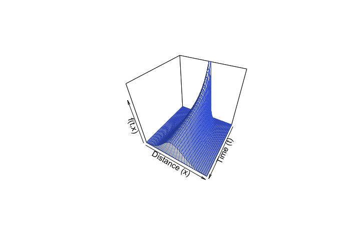Figure 8.7: Heat equation 3D perspective

D = 0.001; r=0.5; L=2; N=40; lambda = 0.3 # discretized factor 
dx = L/(N+1); dt = lambda*(dx*dx)/D; c1 = D*dt/(dx*dx);
yold = rep(0, N+2); ynew = rep(0, N+2);

# initial f(x,t)
x = dx*c(0:(N+1)); 
for(j in 1:(N+2)){ 
 xx = x[j];   
 if (xx<4*L/10) {  
  yold[j] = 0;   }   
 else if (xx<L/2) { 
  yold[j] = (xx-4*L/10)/(4*L/10);   }  
 else if (xx<6*L/10){     
  yold[j] = (6*L/10 - xx)/(4*L/10);   }   
 else { yold[j] = 0} 
}

# plot the initial
plot(yold, col=rgb(65/255,105/255,225/255), type="l", ylim=c(0,0.2), ylab="y")


# heat equation
tend = 50; t = dt;
timeinv = seq(t,tend,by=dt) 
y = matrix(0, nrow=length(timeinv), ncol=N+2); 
y[1,] = yold; 
for(t in timeinv){   
 ynew[1] = yold[1] + c1*(-2*yold[1] + 2*yold[2]);   
 ynew[2:(N+1)] = yold[2:(N+1)] + c1*(yold[1:N] - 2*yold[2:(N+1)] + yold[3:(N+2)]) ;   
 ynew[N+2] = yold[N+2] + c1*(2*yold[N+1] - 2*yold[N+2]);   
 y[t,] = ynew;   
 yold = ynew; 
}

# plot
library(plot3D)
persp3D(z=y[timeinv,], along="y", curtain=TRUE, theta=120, 
space=0.8, shade=0.2, facets = FALSE, col = "royalblue", xlab="Time (t)", ylab="Distance (x)", zlab="f(t,x)")

Figure 8.7 plots the solution in the 3D coordinates \((t,x,f(t,x))\). By fixing \(t\), we can see the change of \(f(t,\cdot)\) across the distance \(x\). By fixing \(x\), we can see the evolution of \(f(\cdot,x)\). In this 3D object, the roles of time and space are simply arguments of the function. For any combinatoric \((t,x)\), one can find the corresponding value \(f(t,x)\) in the graph. The initial \(f(0,x)\) in the plot is given as a spike shape in the middle. Along the time arrow of \(t\), the spike shape becomes flatter (see animation in figure 8.6). This phenomenon is called diffusion, a process combining the temporal and spatial differences. One can imagine that a radiator locates at the center of the room. In the beginning, the heat is concentrated around the radiator, but gradually, the heat diffuses across the room. Eventually, we may expect the temperature of the whole room to increase.

Figure 8.8: 2019-nCoV affected cases

The pioneered applications of the diffusion process beyond physics originate from modeling epidemic in 1950s. We can easily find the diffusive feature from the epidemic data. Here is a recent dataset of the corona-virus. (source: https://www.kaggle.com/sudalairajkumar/novel-corona-virus-2019-dataset ) The disease spread takes place through personal contacts (person-to-person spread). The virus identified as the cause of an outbreak of respiratory illness was first detected in Hubei, a province located in the central part of China. From figure 8.8, one can see that the disease quickly and severely affected a large number of people in central China, then spread to the rest part of China, later to the world.

Similar to the epidemic models, we can regard diffusion as resulting from the spread of information. The information spread takes place through personal contacts like the spread of an epidemic. The key media underlying the epidemic model is information transmission guiding the diffusion path, which is understood to be a self-propagating adjustment process. In the initial phases, the adoption rate is slow due to the lack of information. As information spreads, the rate of adoption speeds up over time, leading eventually to a phase where all the potential communicators receive the information. The same argument holds for knowledge diffusion. The diffusion of new knowledge broadly refers to the mechanism or process that spreads the ideas across social structures such as individuals, firms, or societies. This process is pivotal as without being spread, the new knowledge would have little social impact. The diffusion of knowledge also leads to a period of rapid economic growth.120120 In history, when new products were introduced, there is an intense amount of research and development, which leads to dramatic improvements in quality and reductions in cost. The owners of these new products, at the time of their occurrences, stand in sharp contrast to the great mass of their contemporaries. Every advance first comes into being innovation developed by one or a few persons, only to become, after a time, the indispensable necessity taken for granted by the majority. This diffusion procedure is similar to the evolutionary pattern of \(f(t,\cdot)\) plotted in figure 8.6. The initial spike (in blue) spreads itself to the neighbor region and gradually becomes diffusive (blue turns into red).

The spatial aspect of diffusion is inextricably linked to the rate and speed of diffusion, and the temporal aspect is linked to the sustainable level. With the high degree of integration of world economies, the diffusion model can provide a wide appeal to model the indicating forces of globalization, technological revolution, and conflicts. Conceptualization of the spread across a landscape is primarily the outcome of a learning or communication process. Information flows in a hierarchical way, from the majors (urban centers) to the minors (secondary centers), and if the information sustains long enough, it can transmit in the neighborhood of every “infected” locality. This pattern of diffusion, at the most basic level, forms a source of conceptualizing a hierarchy of networks of social communications, while at a more complex level, the conceptualization can be understood to indicate how well the integration or agglomeration has been formed.