10 Vector and Matrix
We don’t add an apple to orange because they are different fruits. Similarly, the values of two different unknowns \(x_{1}\) and \(x_{2}\) from a linear system \[\begin{equation} \begin{cases} 0.3x_{2}+0.6x_{1} & =1,\\ 0.6x_{2}-0.3x_{1} & =0. \end{cases} \tag{10.1} \end{equation}\] should be treated separately as we did it for the ordered list \((x_{1},x_{2})\in\mathbb{R}^{2}\). The solution \((4/3,\,2/3)\) can be viewed as the point on the plane where two equations intersect (figure 10.1). The notation of \((x_{1},x_{2})\) is free to express any point on the plane. The introduction of a great workable literal symbolism was a significant advance in mathematics. Descartes illustrated his entire scheme of geometry on the Cartesian system of coordinates. This illustration connected algebra to classical geometry.
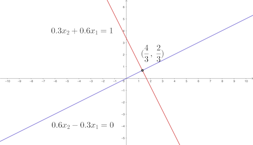 Figure 10.1: System of two equations
However, the geometrical approach becomes impractical when the linear system includes more than three knowns. Graphing in four (or more) dimensions on a flat sheet of paper does not lead to accurate answers. But Descartes’ achievement inspired Leibniz’s dream of symbolism for all of the human thought, in which all arguments about truth or falsehood could be resolved by the computations of symbols. Leibniz argued that such symbolism would relieve the imagination.
To initiate our journey to the imaginary world of symbols, let’s take a closer look at the system (10.1). The useful information of this system is stored by the coefficients on the left-hand side of the equality and by the output values on the right-hand side. The following two tables can compactly list all the necessary information: \[\left[\begin{array}{cc} 0.3 & 0.6\\ 0.6 & -0.3 \end{array}\right],\:\left[\begin{array}{c} 1\\ 0 \end{array}\right].\] There is no need to write out all the equal signs or plus signs. These rectangular tables of numbers are handy in representing the system of equations. The first rectangular table of numbers represents a symbol called the matrix, and the second represents a symbol called the vector. They are the primary objects for studying a general linear system with an arbitrary number of unknowns. By relieving our imagination, we can reduce high-dimensional thought processes to some easily mastered manipulations of symbols.
10.1 Vector
 Figure 10.2: Vector
If we look at the point \((a_{1},a_{2})\in \mathbb{R}^{2}\) of the plane in figure 10.2, there is a line going from the origin to it. Two characteristics of this point, its length and its direction, have been automatically stored in this ordered list. If we scale this line by \(c\), then the point will move to \((ca_{1},ca_{2})\); and if we add another \((b_{1},b_{2})\) to this point, there will be a new ordered list \((a_{1}+b_{1},\, a_{2}+b_{2})\).152 The order does not matter for the addition as \((a_{1}+b_{1},\, a_{2}+b_{2})\) and \((b_{1}+a_{1},\, b_{2}+a_{2})\) are the same.
Let’s relieve our imagination to an ordered list of \(n\) elements. Even it is hard to imagine what is an \(n\)-dimensional space, we may imagine that the direction, length, simple operations such as addition and scalar multiplication should hold as those in \(\mathbb{R}^{2}\). Let’s formally call this \(n\)-dimensional ordered list a vector. Usually, a vector is expressed in a lower-case boldface letter; for displaying the entries or elements of a vector, one can use an vertical array (column vector) surrounded by square (or curved) brackets: \[\mathbf{a}=\left[\begin{array}{c} a_{1}\\ \vdots\\ a_{n} \end{array}\right],\;\mathbf{b}=\left[\begin{array}{c} b_{1}\\ \vdots\\ b_{n} \end{array}\right],\quad\mathbf{a}+\mathbf{b}=\left[\begin{array}{c} a_{1}+b_{1}\\ \vdots\\ a_{n}+b_{n} \end{array}\right],\; c\mathbf{a}=\left[\begin{array}{c} c\times a_{1}\\ \vdots\\ c\times a_{n} \end{array}\right].\]
Like the addition of 2D order lists, when we add one vector to another vector, the addition should take into account the order of the entires of these vectors. Each entry or component of the vector is called the scalar. when we scale the vector by some scalar \(c\), this scalar should multiple all components of the vector. The vector \(\mathbf{a}\in \mathbb{R}^n\) is of size \(n\), and it is called the \(n\)-vector. Two equivalent vectors \(\mathbf{a}\) and \(\mathbf{b}\), namely \(\mathbf{a}=\mathbf{b}\), implies that they have the same size and the same corresponding entries.
The arithmetic axioms or the algebra axioms of vectors are similar to those rules of real numbers. Suppose that \(\mathbf{a}\), \(\mathbf{b}\), and \(\mathbf{c}\) are \(n\)-vectors, namely being of the same size, and suppose that \(k\) and \(l\) are scalars, the axioms can be summarized as follows:
- addition \(+\) (or called commutative group)153 The commutative group is a concept from abstract algebra. The commutative group generalizes the operations that perform similarly as the arithmetic of addition of integers. Here \(+\) operation stands for the operation defining the abstract commutative group rather than the simple addition of integers. That is, if we replace \(\mathbf{a}, \mathbf{b}\in\mathbb{R}^n\) with \(a, b\in\mathbb{Z}\), the axioms still hold. Moreover, if we use some other objects instead of vector \(\mathbf{a}, \mathbf{b}\), and if those objects are from a commutative group, they should also satisfy the axioms regarding this \(+\) operation.:
- commutativity : \(\mathbf{a}+\mathbf{b}=\mathbf{b}+\mathbf{a}\)
- associativity : \((\mathbf{a}+\mathbf{b})+\mathbf{c}=\mathbf{a}+(\mathbf{b}+\mathbf{c})\)
- existence of zero vector (existence of an identity element) : \(\mathbf{a}+\mathbf{0}=\mathbf{a}\)
- existence of negative vector (existence of inverse elements) : \(\mathbf{a}+(-\mathbf{a})=\mathbf{0}\)
- scalar multiplication \(\times\) (We often ignore the sign of scalar multiplication.):
- associativity : \(k(l\mathbf{a})=(k\times l)\mathbf{a}\)
-
multiplication of identity elements :
- one (identity element for multiplication) \(1\mathbf{a}=\mathbf{a}\),
- zero (identity element for addition)\(0\mathbf{a}=\mathbf{0}\),
- and zero vector (identity element for vector addition): \(k\mathbf{0}=\mathbf{0}\)
- distributivity for vectors and for scalars: \(k(\mathbf{a}+\mathbf{b})=k\mathbf{a}+k\mathbf{b}\), \((k+l)\mathbf{a}=k\mathbf{a}+l\mathbf{a}\)
These axioms (commutativity, associativty, negative vector) in 2D can be easily verified by figure 10.2. Note that zero vector \(\mathbb{R}^n\) is the origin in the \(n\)-dimension. Note that a standard unit vector is a vector with all zero elements except one unit element. For example, \[\mathbf{e}_{1}=\left[\begin{array}{c} 1\\ 0\\ 0 \end{array}\right],\:\mathbf{e}_{2}=\left[\begin{array}{c} 0\\ 1\\ 0 \end{array}\right],\:\mathbf{e}_{3}=\left[\begin{array}{c} 0\\ 0\\ 1 \end{array}\right]\] are the three standard unit vectors in \(\mathbb{R}^{3}\).
 Figure 10.3: Represent a 3D vector in a linear combination
A linear combination is formed by combining some additions and scalar multiplications of some vectors. Let \(\mathbf{x}_{1},\dots,\mathbf{x}_{m}\) be \(n\)-vectors, and let \(\beta_{1},\dots,\beta_{m}\) be scalars, then the \(n\)-vector \[\beta_{1}\mathbf{x}_{1}+\cdots+\beta_{m}\mathbf{x}_{m}\] is a linear combination of the vectors \(\mathbf{x}_{1},\dots,\mathbf{x}_{m}\). The scalars \(\beta_{1},\dots,\beta_{m}\) are the coefficients of this linear combination. We can write any \(n\)-vector \(\mathbf{x}\) as a linear combination of the standard unit vectors,\[\mathbf{x}=x_{1}\mathbf{e}_{1}+\cdots+x_{n}\mathbf{e}_{n}\] where \(x_{i}\) is the \(i\)-th entry of \(\mathbf{x}\), and \(\mathbf{e}_{i}\) is the \(i\)-th standard unit vector. A 3D illustration of the linear combination is given in figure 10.3.
An essential aspect we didn’t mention is about the multiplication or the product of two vectors. As any vector stores the relevant information of direction and length, the product should preserve the metric information, i.e., the measurement of the angles and the lengths of the vectors. The length of an \(n\)-vector \(\mathbf{x}\) is given by the Euclidean distance from the origin \[\mbox{d}(\mathbf{x},\mathbf{0})=\sqrt{x_{1}^{2}+\cdots+x_{n}^{2}}=\|\mathbf{x}\|\in\mathbb{R}\] where \(\|\cdot\|\) denotes a norm, a function that assigns a strictly positive length to a vector. The norm of the vector \(\mathbf{x}\) is equivalent to the \(l_{2}\)-distance function for \(\mathbf{x}\) and \(\mathbf{0}\), namely \(\mbox{d}(\mathbf{x},\mathbf{0})\). For zero vector, the length is also zero, thus \(\|\mathbf{0}\|=0\).154 The norm is induced by the distance, i.e. \(\mbox{d}(\mathbf{x},\mathbf{y})=\|\mathbf{x}-\mathbf{y}\|\). Different norms associate with different distance functions, but not all distance functions come from norms (see chapter 15.1).
The product of two vectors is called the inner product, and can be defined as follows: \[\begin{equation} \langle\mathbf{a},\,\mathbf{b}\rangle=a_{1}b_{1}+\cdots+a_{n}b_{n}=\sum_{i=1}^{n}a_{i}b_{i}. \tag{10.2} \end{equation} \] On the other hand, one can also define the inner product by \[\begin{equation} \langle\mathbf{a},\,\mathbf{b}\rangle= \begin{cases} \|\mathbf{a}\|\|\mathbf{b}\|\cos\theta, & \mbox{ if }\mathbf{a},\mathbf{b}\neq0,\\ 0, & \mbox{ if }\mathbf{a}=0,\mbox{ or }\mathbf{b}=0, \end{cases} \tag{10.3} \end{equation} \] where \(\theta\) is the smallest angle between \(\mathbf{a}\) and \(\mathbf{b}\). These two definitions are equivalent.
Proof
Expression (10.2) to expression (10.3)
If either \(\mathbf{a}=0\) or \(\mathbf{b}=0\), then \(\sum_{i=1}^{n}a_{i}b_{i}=0\) and \(\|\mathbf{a}\|\|\mathbf{b}\|=0\). Thus two expressions give the same answer.
For a non-zero inner product, let’s first consider the case in \(\mathbb{R}^2\). Any vector satisfying \(\|\mathbf{x}\|=1\) is a unit vector (not necessarily being a standard unit vector). Note that the vector \(\mathbf{u}\) satisfying \[\mathbf{u}=\left[\begin{array}{c} \cos\theta\\ \sin\theta \end{array}\right],\:\|\mathbf{u}\|=\sqrt{\cos^{2}\theta+\sin^{2}\theta}=1\] is a unit vector. The unit vector \(\mathbf{u}\) and another unit vector \(\mathbf{u}'\) have the inner product of their angle differences \[\langle\mathbf{u},\,\mathbf{u}'\rangle=\cos\theta\times\cos\theta'+\sin\theta\times\sin\theta'=\cos(\theta-\theta')\] by the trigonometry formula.155 When \(\theta'=0\), the unit vector \(\mathbf{u}'\) is the standard unit vector \(\mathbf{e}_{1}\). Then \(\mathbf{u}\) and the standard unit vector \(\mathbf{e}_{1}\) has the inner product \[\langle\mathbf{u},\,\mathbf{e}_{1}\rangle=\cos\theta\times1+\sin\theta\times0=\cos\theta.\] Thus we can conclude that for any two unit vectors in \(\mathbb{R}^2\), the two definitions of the inner product are equivalent.
Now consider the general case in \(\mathbb{R}^n\). It is always true that \(\mathbf{a}/\|\mathbf{a}\|\) and \(\mathbf{b}/\|\mathbf{b}\|\) are unit vectors.156 Take \(\mathbf{a}/\|\mathbf{a}\|\) as an example. \[\begin{align*} \left\Vert \frac{\mathbf{a}}{\|\mathbf{a}\|}\right\Vert =&\sum_{i=1}^{n}\frac{1}{\|\mathbf{a}\|}\left(a_{1}^{2}+\cdots+a_{n}^{2}\right)\\ =&\frac{1}{\|\mathbf{a}\|}\sum_{i=1}^{n}\left(a_{1}^{2}+\cdots+a_{n}^{2}\right) \\= &\frac{1}{\|\mathbf{a}\|}\|\mathbf{a}\|=1. \end{align*}\] Transforming \(\mathbf{a}\) into \(\mathbf{a}/\|\mathbf{a}\|\) is called the normalization of the vector \(\mathbf{a}\). Therefore, trigonometry formula tells us \[\left\langle \frac{\mathbf{a}}{\|\mathbf{a}\|},\,\frac{\mathbf{b}}{\|\mathbf{b}\|}\right\rangle =\cos\theta\] which implies \(\langle\mathbf{a},\,\mathbf{b}\rangle=\|\mathbf{a}\|\|\mathbf{b}\|\cos\theta.\) The result follows.157 Note that \[\begin{align*}\left\langle \frac{\mathbf{a}}{\|\mathbf{a}\|},\,\frac{\mathbf{b}}{\|\mathbf{b}\|}\right\rangle =&\frac{1}{\|\mathbf{a}\|\|\mathbf{b}\|}\sum_{i=1}^{n}a_{i}b_{i}\\=&\frac{\langle\mathbf{a},\,\mathbf{b}\rangle}{\|\mathbf{a}\|\|\mathbf{b}\|}.\end{align*}\]
There is also an alternative way of expressing an inner product as a product of a row vector and a column vector. See chapter 10.3.
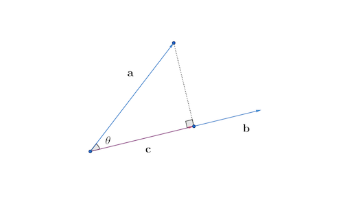 Figure 10.4: Projection
The expression (10.3) can imply several important results. If \(\langle\mathbf{a},\,\mathbf{b}\rangle=0\) in equation (10.2) and \(\mathbf{a},\mathbf{b}\neq0\), then the expression (10.3) says that \(\mathbf{a}\) and \(\mathbf{b}\) must be perpendicular (orthogonal to each other), namely \(\theta=90^{\circ}\). Also, since \(|\cos\theta|\) never exceeds one, expression (10.3) gives the following inequality \[\left|\frac{\langle\mathbf{a},\,\mathbf{b}\rangle}{\|\mathbf{a}\|\|\mathbf{b}\|}\right|\leq1,\;\mbox{ or say}\left|\langle\mathbf{a},\,\mathbf{b}\rangle\right|\leq\|\mathbf{a}\|\|\mathbf{b}\|,\] which is called Schwarz inequality. Because the norm \(\|\cdot\|\) is a distance function, it should also satisfy the triangular inequality \[\|\mathbf{a}+\mathbf{b}\|\leq\|\mathbf{a}\|+\|\mathbf{b}\|.\] Finally, by the expression (10.3), we can deduce a useful formula called the orthogonal projection formula. Consider a situation in which one vector \(\mathbf{a}\) shall be projected orthogonally onto another vector \(\mathbf{b}\) in order to create a new vector \(\mathbf{c}\). Since \(\mathbf{a}\) and \(\mathbf{c}\) make up a triangle with a right angle (see figure 10.4), by the definition of cosine function, we have \(\cos\theta=\|\mathbf{c}\|/\|\mathbf{a}\|\) or \(\|\mathbf{c}\|=\cos\theta\|\mathbf{a}\|\). Then by normalizing \(\mathbf{b}\) and \(\mathbf{c}\), we have \(\mathbf{c}/\|\mathbf{c}\|=\mathbf{b}/\|\mathbf{b}\|\), and hence \[\mathbf{c}=\|\mathbf{c}\|\frac{\mathbf{b}}{\|\mathbf{b}\|}=\|\mathbf{a}\|\cos\theta\frac{\mathbf{b}}{\|\mathbf{b}\|}.\] By the definition of inner product (expression (10.3)), we have \[ \begin{equation} \mathbf{c}=\|\mathbf{a}\|\|\mathbf{b}\|\cos\theta\frac{\mathbf{b}}{\|\mathbf{b}\|^{2}}=\frac{\langle\mathbf{a},\,\mathbf{b}\rangle}{\|\mathbf{b}\|^{2}}\mathbf{b}. \tag{10.4} \end{equation} \] The term \(\langle\mathbf{a},\,\mathbf{b}\rangle/\|\mathbf{b}\|^{2}\) gives the orthogonal projection of \(\mathbf{a}\) onto \(\mathbf{b}\).158 Note that \(\|\mathbf{b}\|^{2}=\langle\mathbf{b},\,\mathbf{b}\rangle\), one can also write the ** orthogonal projection** of \(\mathbf{a}\) onto \(\mathbf{b}\) as \[\frac{\langle\mathbf{a},\,\mathbf{b}\rangle}{\langle\mathbf{b},\,\mathbf{b}\rangle}\mathbf{b}\].
With the projection formula (10.4), we can deduce the following rules (axioms).
- Rules of inner product \(\langle\cdot,\,\cdot\rangle\) for \(\mathbf{a},\mathbf{b}\in\mathbb{R}^{n}\) and \(k\in\mathbb{R}\):
- Commutativity : \(\langle\mathbf{a},\,\mathbf{b}\rangle=\langle\mathbf{b},\,\mathbf{a}\rangle\)
- Associativity : \(k\langle\mathbf{a},\,\mathbf{b}\rangle=\langle k\mathbf{a},\,\mathbf{b}\rangle=\langle\mathbf{a},\, k\mathbf{b}\rangle\)
- Distributivity : \(\langle\mathbf{a},\,\mathbf{b}+\mathbf{c}\rangle=\langle\mathbf{a},\,\mathbf{b}\rangle+\langle\mathbf{a},\,\mathbf{c}\rangle\)
Proof
 Figure 10.5: Distributivity
Commutativity and associativity come directly from the definition (10.2) and (10.3). To see distributivity, we need to see that the sum of the projections is equal to the projection of the sum, (figure 10.5). It means\[\frac{\langle\mathbf{b}+\mathbf{c},\,\mathbf{a}\rangle}{\|\mathbf{a}\|^{2}}\mathbf{a}=\frac{\langle\mathbf{b},\,\mathbf{a}\rangle}{\|\mathbf{a}\|^{2}}\mathbf{a}+\frac{\langle\mathbf{c},\,\mathbf{a}\rangle}{\|\mathbf{a}\|^{2}}\mathbf{a}.\] We only need to focus on the coefficients of this equality. By canceling out \(\|\mathbf{a}\|^{2}\) on the both sides, we have \[\langle\mathbf{b}+\mathbf{c},\,\mathbf{a}\rangle=\langle\mathbf{b},\,\mathbf{a}\rangle+\langle\mathbf{c},\,\mathbf{a}\rangle.\] Then interchanging the positions of \(\mathbf{a}\) by the commutativity rule gives the desired result.
As the expression (10.2) defines a Euclidean distance for two \(n\)-vectors \(\mathbf{a}\) and \(\mathbf{b}\), the inner product is a particular type of distance. Note that the five axioms of distance functions do not include everything that can be said about distance in our common sense of geometry. Pythagoras’ theorem, for instance, cannot be deduced from those five axioms but it can be deduced by the rules of inner product. If \(\mathbf{a}\) and \(\mathbf{b}\) are orthogonal to each other, then \[\|\mathbf{a}+\mathbf{b}\|^{2}=\|\mathbf{a}\|^{2}+\|\mathbf{b}\|^{2}\] gives a generalized Pythagoras’ theorem.159 \[ \begin{align*} \|\mathbf{a}+\mathbf{b}\|^{2}&= \langle\mathbf{a}+\mathbf{b},\,\mathbf{a}+\mathbf{b}\rangle\\ &\overset{(a)}{=} \langle\mathbf{a},\,\mathbf{a}+\mathbf{b}\rangle+\langle\mathbf{b},\,\mathbf{a}+\mathbf{b}\rangle\\ &\overset{(b)}{=} \langle\mathbf{a},\,\mathbf{a}\rangle+\langle\mathbf{a},\,\mathbf{b}\rangle+\langle\mathbf{b},\,\mathbf{a}\rangle+\langle\mathbf{b},\,\mathbf{b}\rangle\\ &= \|\mathbf{a}\|^{2}+\|\mathbf{b}\|^{2}+2\langle\mathbf{a},\,\mathbf{b}\rangle\\ &\overset{(c)}{=}\|\mathbf{a}\|^{2}+\|\mathbf{b}\|^{2} \end{align*} \] where \(\overset{(a)}{=}\) and \(\overset{(b)}{=}\) use the distributive rule, \(\overset{(c)}{=}\) use the orthogonality \(\langle\mathbf{a},\,\mathbf{b}\rangle=0\). In this sense, the definition of inner product (expression (10.3)) actually specifies the projective geometry properties of vectors.
10.2 Example: Linearity
Vectors establish the basic objects in the numerical computation. Consider a function \(f:\mathbb{R}^{n}\mapsto\mathbb{R}\). We can model this function by saying that it maps from real \(n\)-vectors to real numbers such as \(f(\mathbf{x})=f(x_{1},\dots,x_{n})\). And the inner product is such a function:\[f(\mathbf{x})=\langle\mathbf{b},\,\mathbf{x}\rangle=b_{1}x_{1}+\cdots+b_{n}x_{n}\] where \(b_{1},\dots,b_{n}\) are the coefficients. The inner product can uniquely represent a class of functions called linear functions. The linear function is one of the most fundamental functions. For example, in economics, the total income or the total expenses can be expressed by an inner product of quantities and prices of \(n\) items.
A function \(f\) is linear or superposition if \[f(\alpha x+\beta y)=\alpha f(x)+\beta f(y)\] for scalars \(\alpha\) and \(\beta\). The property \(f(\alpha x)=\alpha f(x)\) is called the homogeneity, and the property \(f(x+y)=f(x)+f(y)\) is called the additivity.160 We can easily find that if the linear function is an inner product, then the aditivity and homogeneity are respectively corresponding to the rules of addition and scalar multiplication of vectors. Combining homogenity and additivity gives the superposition. For any function \(f:\mathbb{R}^{n}\mapsto\mathbb{R}\), if \(f\) is linear, then \(f\) can be uniquely represented by an inner product of its argument \(\mathbf{x}\in\mathbb{R}^{n}\) with some fixed vector \(\mathbf{b}\in\mathbb{R}^{n}\), namely \(f(\mathbf{x})=\langle\mathbf{b},\,\mathbf{x}\rangle\).
Proof
Multi-valued function
The vector also allows us to study some function mapping to higher dimensions \(\mathbf{f}:\mathbb{R}\mapsto\mathbb{R}^{n}\). For example, the dynamical 3D spiral in figure 4.6 is such a function \[\mathbf{f}(t)=\left[\begin{array}{c} f_{1}(t)\\ f_{2}(t)\\ f_{3}(t) \end{array}\right]=\left[\begin{array}{c} \mbox{e}^{t}\cos t,\\ \mbox{e}^{t}\sin t\\ t \end{array}\right].\] The continuity for \(\mathbf{f}:\mathbb{R}\mapsto\mathbb{R}^{n}\) should take into account the continuity in each dimension, namely the continuity of every \(f_{i}(x)\) in the vector \(\mathbf{f}(x)\). The limit \(\lim_{x\rightarrow a}\mathbf{f}(x)\) does not exists if and only if there is a sequence \(x_{n}\rightarrow a\) such that \(\mathbf{f}(x_{n})\) does not converge. The function \(\mathbf{f}(x)\) is continuous at a point \(a\) if \(\lim_{x\rightarrow a}\mathbf{f}(x)=\mathbf{f}(a)\).
Gradient
With the properties of function values in \(\mathbb{R}^n\), let’s consider a special mapping from \(\mathbb{R}^{n}\) to \(\mathbb{R}^{n}\) which is called the gradient. Consider a differentiable function \(f:\mathbb{R}^{n}\mapsto\mathbb{R}\), the gradient of \(f\) is an \(n\)-vector \[\nabla f(\mathbf{z})=\left[\begin{array}{c} \left.\frac{\partial f}{\partial x_{1}}(\mathbf{x})\right|_{\mathbf{x}=\mathbf{z}}\\ \vdots\\ \left.\frac{\partial f}{\partial x_{n}}(\mathbf{x})\right|_{\mathbf{x}=\mathbf{z}} \end{array}\right]\] where \(\partial f/\partial x_{i}\) is the partial derivative \[\frac{\partial f}{\partial x_{i}}(\mathbf{x})=\lim_{\epsilon\rightarrow0}\frac{f(x_{1},\dots,x_{i}+\epsilon,\dots x_{n})-f(\mathbf{x})}{\epsilon}.\] We can linearize a nonlinear (vector) function \(f:\mathbb{R}^{n}\mapsto\mathbb{R}\) by Taylor series such that \[f(\mathbf{x})\approx f(\mathbf{z})+\left\langle \nabla f(\mathbf{z}),\,(\mathbf{x}-\mathbf{z})\right\rangle.\] The first term in the Taylor series is a constant vector \(f(\mathbf{z})\), the second term is the inner product of the gradient of \(f\) at \(\mathbf{z}\) and the difference between \(\mathbf{x}\) and \(\mathbf{z}\). This first order Taylor expansion is a linear function \(\left\langle \nabla f(\mathbf{z}),\,(\mathbf{x}-\mathbf{z})\right\rangle\) plus a constant vector \(f(\mathbf{z})\).161 A linear function \(\langle\mathbf{b},\,\mathbf{x}\rangle\) plus a constant vector \(\mathbf{a}\) is called an affine function \(f(\mathbf{x})=\langle\mathbf{b},\,\mathbf{x}\rangle+\mathbf{a}\). In many applied contexts affine functions are also called linear functions. However, in order to satisfy the superposition property, the argument \(\alpha x+\beta y\) should satisfy \(\alpha+\beta=1\). To see this, note that \[\begin{align*} f(\alpha\mathbf{x}+\beta\mathbf{y}) &= \langle\mathbf{b},\,\alpha\mathbf{x}+\beta\mathbf{y}\rangle+\mathbf{a}\\ &= \alpha\langle\mathbf{b},\,\mathbf{x}\rangle+\beta\langle\mathbf{b},\,\mathbf{y}\rangle+\mathbf{a}. \end{align*}\] Using the property \(\alpha+\beta=1\), the previous expression becomes \[\begin{align*} \alpha\langle\mathbf{b},\,\mathbf{x}\rangle+\beta\langle\mathbf{b},\,\mathbf{y}\rangle+&(\alpha+\beta)\mathbf{a} =\\ \alpha(\langle\mathbf{b},\,\mathbf{x}\rangle+\mathbf{a})+&\beta(\langle\mathbf{b},\,\mathbf{y}\rangle+\mathbf{a})\\ = \alpha f(\mathbf{x})+\beta f(\mathbf{y}). \end{align*}\]
Fixed point of vectors
Let’s look at a vector version fixed point result. The previous system (10.1) can be rewritten as \[\begin{align*} \mathbf{x}=&\left[\begin{array}{c} x_{1}\\ x_{2} \end{array}\right] =\left[\begin{array}{c} 0.4x_{1}-0.3x_{2}+1\\ 0.3x_{1}+0.4x_{2} \end{array}\right]\\ &=\left[\begin{array}{c} 1\\ 0 \end{array}\right] +\left[\begin{array}{c} g_{1}(\mathbf{x})\\ g_{2}(\mathbf{x}) \end{array}\right]=\mathbf{d}+\mathbf{g}(\mathbf{x})=\mathbf{f}(\mathbf{x}) \end{align*}\] where \(\mathbf{g}:\mathbb{R}^{2}\mapsto\mathbb{R}^{2}\) is a linear function (both \(g_{1}\) and \(g_{2}\) are linear), and \(\mathbf{f}:\mathbb{R}^{2}\mapsto\mathbb{R}^{2}\) is an affine function. The following simple code shows that the system reach the point around \(x_{1}=4/3\) and \(x_{2}=2/3\), namely the solution vector of the linear system.
x1 = 0; x2 = 0;
for (iter in 1:10){
  x1 = 0.4*x1 - 0.3*x2 + 1 ;
  x2 = 0.3*x1 + 0.4*x2;
  cat("At iteration", iter, "x1 is:", x1, "x2 is:", x2, "\n")
}
## At iteration 1 x1 is: 1 x2 is: 0.3
## At iteration 2 x1 is: 1.31 x2 is: 0.513
## At iteration 3 x1 is: 1.3701 x2 is: 0.61623
## At iteration 4 x1 is: 1.363171 x2 is: 0.6554433
## At iteration 5 x1 is: 1.348635 x2 is: 0.6667679
## At iteration 6 x1 is: 1.339424 x2 is: 0.6685343
## At iteration 7 x1 is: 1.335209 x2 is: 0.6679765
## At iteration 8 x1 is: 1.333691 x2 is: 0.6672978
## At iteration 9 x1 is: 1.333287 x2 is: 0.6669052
## At iteration 10 x1 is: 1.333243 x2 is: 0.666735From the result table, we can see that the Lipschitz continuity is satisfied for this affine function. \[\|\mathbf{f}(\mathbf{x})-\mathbf{f}(\mathbf{x}')\|\leq\|\mathbf{x}-\mathbf{x}'\|.\] The sequence is a Cauchy sequence.
For a general case, let the fixed point of the system of two equations \(x_1=f_{1}(x_1,x_2),\; x_2=f_{2}(x_1,x_2)\) be \((x_1^{*},x_2^{*})\) such that \(x_1^{*}=f_{1}(x_1^{*},x_2^{*})\) and \(x_2^{*}=f_{2}(x_1^{*},x_2^{*})\). The fixed-point iteration is \[x_1^{(k+1)}=f_{1}(x_1^{(k)},x_2^{(k)}),\; x_2^{(k+1)}=f_{2}(x_1^{(k)},x_2^{(k)}).\] Their paritial derivatives are continuous on a region that contains the fixed point \((x_1^{*},x_2^{*})\). If \((x_1,x_2)\) is sufficiently close to \((x_1^{*},x_2^{*})\) and if \[\left|\frac{\partial f_{i}}{\partial x_1}(x_1^{*},x_2^{*})\right|+\left|\frac{\partial f_{i}}{\partial x_2}(x_1^{*},x_2^{*})\right|<1\] for \(i=1,2\), then the iteration converges stably to \((x_1^{*},x_2^{*})\).162 Otherwise, the iteration might diverge. This will usually be the case if the sum of the magnitudes of the partial derivatives is much larger than \(1\). See chapter 8.4 for the discussion about the stability of fixed point algorithms.
Linear regression
Very often, besides the input and the output, the system is also characterized by the parameters. To be precise, we recall the notion of the regression \(g(X)=\mathbb{E}[Y|X]\), a conditional expectation with the output \(Y\) and the (conditional) input \(X\). If we let \(Y\) be a linear function with an additive i.i.d. random variable \(\varepsilon\) and a parameter \(\beta\) as the coefficient of this linear function such that \[Y=\beta X+\varepsilon,\] then the regression is a linear regression, or say \(g(X)=\beta X\) as \(\mathbb{E}[\varepsilon|X]=0\) for the i.i.d. random variable.
When the parameter \(\beta\) is unknown, we need to estimate the value of \(\beta\) through the sequences of observations of \(X\) and \(Y\). That is, we want to determine the model parameters that produce the observable data we have recorded. This problem is known as the estimation problem: one looks for the model parameter that presumably generates the data. In data analysis, the observations (realizations) of a random variable \(X\) (or \(Y\)) are stored by an array, namely the data vector \(\mathbf{x}\) (or \(\mathbf{y}\)).
 Figure 10.6: Least square estimate
The table displays ten observations for \(X\) and \(Y\). These are \(10\)-vector \(\mathbf{x}\) and \(10\)-vector \(\mathbf{y}\). These vectors are generated by a Monte Carlo simulation. The parameter recovery simulations have frequently been used to assess the accuracy of the estimation. We assume that a model accurately captures the processes that generate data, and fit the model to the data so as to draw conclusions from its parameter estimates.
A very commonly used estimation method for linear regression models is the least square method. The name of least square comes from the fact that the method minimizes the (square of the) error \(\mathbf{y} - \beta \mathbf{x}\) by tuning the value of \(\beta\). The unique value of \(\beta\) should match the data better than the others.
We will come back to the minimization point of least square in Ch[?]. At the moment, we can see how to find the best \(\beta\) from the geometric point of view. The preassumbly relation between \(X\) and \(Y\) is linear, so scaling the vector \(\mathbf{x}\) by \(\beta\) unit was supposed to get the vector \(\mathbf{y}\). Due to the contaminations163 In our simulation, the contaminations were added by ten draws from a normal random variable \(\mathcal{N}(0,4)\)), the vector \(\mathbf{y}\) does not stay with \(\mathbf{x}\) at the same plane. We know that when two points \(\mathbf{y}\) and \(\mathbf{x}\) are on different planes, the nearest point to \(\mathbf{x}\) is the projection of \(\mathbf{y}\) onto the plane of \(\mathbf{x}\). The value of \(\beta\) comes from such a projection is the least square estimator, denoted by \(\hat{\beta}\). In other words, we can estimate the parameter \(\beta\) by projecting \(\mathbf{y}\) onto the plane of \(\mathbf{x}\). By the projection formula (10.4), we can deduce the estimator\[\hat{\beta}=\frac{\langle\mathbf{x},\,\mathbf{y}\rangle}{\langle\mathbf{x},\,\mathbf{x}\rangle}\] and the estimated output (the projected output) \(\hat{\beta}\mathbf{x}\). The difference between \(\mathbf{y}\) and \(\hat{\beta}\mathbf{x}\) is called the residual. The residual measures the discrepancy between the data and the estimated model. For any given input \(x\), one can also predict the output through \(\hat{\beta}x\).
## [1] 5.02727210.3 Matrix
A matrix is a rectangular array, with rows and columns, of numbers.164 Strictly speaking, it is a rectangular array of numbers of a field, see Ch[?]. If a matrix has \(m\) rows and \(n\) columns, then the size of the matrix is said to be \(m\times n\) (read \(m\) by \(n\)). We use a boldface capital letter, e.g. \(\mathbf{A}\), to denote a matrix. We write\[\mathbf{A}=[a_{ij}]_{m\times n}\;\mbox{for }1\leq i\leq m,\:1\leq j\leq n,\] where \(a_{ij}\) is the entry in location \((i,j)\), namely stored in the \(i\)-th row and \(j\)-th column of the matrix. In the expanded form, we write\[\mathbf{A}=\left[\begin{array}{ccccc} a_{11} & \cdots & a_{1j} & \cdots & a_{1n}\\ a_{21} & \cdots & a_{2j} & \cdots & a_{2n}\\ \vdots & & & & \vdots\\ a_{i1} & \cdots & a_{ij} & \cdots & a_{in}\\ \vdots & & & & \vdots\\ a_{m1} & \cdots & a_{mj} & \cdots & a_{mn} \end{array}\right].\] As you can see, each column of the \(m\times n\) matrix \(\mathbf{A}\) is an \(m\)-vector \(\mathbf{a}_{j}\) for \(j=1,\dots n\). We can express the matrix as \[\mathbf{A}=[\mathbf{a}_{1},\dots,\mathbf{a}_{n}],\] which is an \(n\)-row vector with \(m\) column vectors as entries. If \(m=1\), then the \(1\times n\) matrix is a row vector; if \(n=1\), then this \(m\times1\) matrix is a (column) vector. If \(m=n\), the matrix is called a squared matrix of order \(n\). In figure 10.7, we can see that a \(3\times3\) matrix is constructed by three 3-vectors.
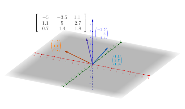 Figure 10.7: Matrix and vectors
Any vector, either a row or a column, can be transposed, which means that a row vector turns into a column vector, and vice versa. Sometimes we define the vector by writing out its elements in the text as a row vector, then using the transpose operator to turn it into a standard column vector, e.g. \(\mathbf{a}=[a_{1},a_{2},a_{3}]^{\top}\). For an \(m\)-columns vector \(\mathbf{a}\), its transposed vector is an \(m\)-rows vector, denoted by \(\mathbf{a}^{\top}=[a_{1},\dots,a_{m}\).] The order of the vector components is preserved. In addition, we can transpose a vector twice, and get back the same vector, i.e., \((\mathbf{a}^{\top})^{\top}=\mathbf{a}\).
With the transpose operation, we can express the inner product \(\langle\mathbf{a},\,\mathbf{b}\rangle\) as the product of \(\mathbf{a}^{\top}\) and \(\mathbf{b}\), such that \[\langle\mathbf{a},\,\mathbf{b}\rangle=\mathbf{a}^{\top}\mathbf{b}=[a_{1},\dots a_{m}]\left[\begin{array}{c} b_{1}\\ \vdots\\ b_{m} \end{array}\right]=\sum_{i=1}^{m}a_{i}b_{i},\] a sum of component-wise multiplications, each \(i\)-th position of the row vector times the \(i\)-th position of the column vector. Note that for the vector \(\mathbf{a}=[a_{1},\dots,a_{m}]^{\top}\), and \(\mathbf{b}^{\top}=[b_{1},\dots,b_{m}]\), \(\mathbf{a}\mathbf{b}^{\top}\) is not a number but a matrix \(\mathbf{C}=[a_{i}b_{j}]_{ij}\).165 In quantum mechanics, it is common to write the inner product \(\langle\mathbf{a},\,\mathbf{b}\rangle\) as \(\langle\mathbf{a}\,|\,\mathbf{b}\rangle\), and write \(\mathbf{a}\mathbf{b}^{\top}\) as \(|\mathbf{a}\rangle\,\langle\mathbf{b}|\) which is called the outer product. The vector \(\mathbf{a}\) is denoted by \(|\mathbf{a}\rangle\), and its transport \(\mathbf{a}^{\top}\) is denoted by \(\langle\mathbf{a}\,|\).
A matrix can also be transposed. The transpose of a matrix is the mirror image of the matrix across the diagonal line. The transpose of an \(m\times n\) matrix \(\mathbf{A}=[a_{ij}]_{m\times n}\) is denoted by \(\mathbf{A}^{\top}=[a_{ji}]_{n\times m}\), i.e.\[\left[\begin{array}{cc} 1 & 2\\ 3 & 4\\ 5 & 6 \end{array}\right]^{\top}=\left[\begin{array}{ccc} 1 & 3 & 5\\ 2 & 4 & 6 \end{array}\right].\] We make the columns of \(\mathbf{A}\) into rows in \(\mathbf{A}^{\top}\) (or rows of \(\mathbf{A}\) into columns in \(\mathbf{A}^{\top}\)).
Let \(\mathbf{A}=[a_{ij}]_{m\times n}\) and \(\mathbf{B}=[b_{ij}]_{m\times n}\) be the matrices of the same size. Then the sum of the matrices, denoted by \(\mathbf{A}+\mathbf{B}\), results another \(m\times n\) matrix: \[\mathbf{A}+\mathbf{B}=\left[\begin{array}{ccc} a_{11}+b_{11} & \cdots & a_{1n}+b_{1n}\\ \vdots & \cdots & \vdots\\ a_{m1}+b_{m1} & \cdots & a_{mn}+b_{mn} \end{array}\right]=[a_{ij}+b_{ij}]_{m\times n}.\] The negative of the matrix \(\mathbf{A}\), denoted by \(-\mathbf{A}\) is \(-\mathbf{A}=[-a_{ij}]_{m\times n}\). Thus the difference of \(\mathbf{A}\) and \(\mathbf{B}\) is \(\mathbf{A}-\mathbf{B}=[a_{ij}-b_{ij}]_{m\times n}\). Notice that both matrices and vectors must be the same size before we attempt to add them. The product of a scalar \(c\) with the matrix \(\mathbf{A}\) is \(c\mathbf{A}=[ca_{ij}]_{m\times n}\). Because the matrix is simply constructed by vectors, the algebraic axioms of the vector, namely addition and scalar mutiplication, also work for the matrix.166 Addition: (commutativity) \(\mathbf{A}+\mathbf{B}=\mathbf{B}+\mathbf{A}\), (associativity) \(\mathbf{A}+(\mathbf{B}+\mathbf{C})=(\mathbf{A}+\mathbf{B})+\mathbf{C}\), (additive inverse) \(\mathbf{A}+(-1)\mathbf{A}=0\). Scalar multiplication: (associativity) \(k(l\mathbf{A})=(kl)\mathbf{A}\), (distributivity) \((k+l)\mathbf{A}=k\mathbf{A}+l\mathbf{A}\), \(k(\mathbf{A}+\mathbf{B})=k\mathbf{A}+k\mathbf{B}\).
While matrix multiplication by a scalar and matrix addition are rather straightforward, the matrix-matrix multiplication may not be so. It is better to consider first the matrix-vector multiplication.
Since any matrix can be expressed as a row vector of column vectors, and since the inner product rule also holds for both types of vectors, we can express the matrix-vector multiplication in terms of inner products. For an \(m\times n\) matrix \(\mathbf{A}=[\mathbf{a}_{1},\dots,\mathbf{a}_{n}]\) and an \(m\)-vector \(\mathbf{b}\), the inner product between \(\mathbf{b}\) and any \(\mathbf{a}_{j}\) for \(j=1,\dots n\) follows the previous definition such that \(\langle\mathbf{b},\,\mathbf{a}_{j}\rangle=\sum_{i=1}^{m}b_{i}a_{ij}\). As the matrix \(\mathbf{A}\) consists of \(n\) components of \(m\)-vector \(\mathbf{a}_{j}\), we need to have the component-wise inner products for all \(\mathbf{a}_{j}\). The result is a row \(n\)-vector \([\sum_{i=1}^{m}b_{i}a_{i1},\dots,\sum_{i=1}^{m}b_{i}a_{in}]\). We can write a compact expression using the transpose operation \[\mathbf{b}^{\top}\mathbf{A}=\left[\mathbf{b}^{\top}\mathbf{a}_{1},\dots,\mathbf{b}^{\top}\mathbf{a}_{n}\right].\] which reads “vector \(\mathbf{b}\) times matrix \(\mathbf{A}\).” For an \(n\)-vector \(\mathbf{x}\), the mutiplication results in\[\mathbf{A}\mathbf{x}=[\mathbf{a}_{1},\dots\mathbf{a}_{n}]\left[\begin{array}{c} x_{1}\\ \vdots\\ x_{n} \end{array}\right]=\mathbf{a}_{1}x_{1}+\cdots+\mathbf{a}_{n}x_{n}\]
which is a linear combination of \(\mathbf{a}_{j}\), \(j=1,\dots,n\). We read “matrix \(\mathbf{A}\) times vector \(\mathbf{x}\)”. Note that \(\mathbf{A}\mathbf{x}\) is a column \(m\)-vector while \(\mathbf{b}^{\top}\mathbf{A}\) is a row \(n\)-vector. As you can see, the inner product restricts the multiplication rule to the case of two vectors with an identical size.167 For \(\mathbf{x}\mathbf{A}\), the size of the row of \(\mathbf{A}\) has to equal to the size of \(\mathbf{x}\). For \(\mathbf{A}\mathbf{x}\), the size of the column of \(\mathbf{A}\) has to equal to the size of \(\mathbf{x}\). Figure 10.8 illustrates how to compute the multiplication of \(\mathbf{A}\mathbf{x}\) by using row-vectors of \(\mathbf{A}\), then calculating the inner products between the row-vectors and \(\mathbf{x}\).168 The numerical entries come from Nine Chapters on the Mathematical Art. In the chapter of the system of equations (Chapter 8), it gives 18 problems and one of them (problem 17 about the costs of a sheep, a dog, a chick and a rabbit) can be expressed in this multiplication.
 Figure 10.8: Illustration of the rule of matrix-vector multiplication
Matrix-vector notation can help us to simplify the operations for linear systems. Recall that a single linear equation \(2x_{1}-3x_{2}+4x_{3}=5\) can be expressed as an inner product: \[[2,-3,4]\left[\begin{array}{c} x_{1}\\ x_{2}\\ x_{3} \end{array}\right]=5.\] The linear system is a collection of linear equations. Consider the following system: \[\begin{equation} \begin{array}{cc} x_{1} & =y_{1},\\ -x_{1}+x_{2} & =y_{2},\\ -x_{2}+x_{3} & =y_{3}. \end{array} \tag{10.5} \end{equation}\] For three vectors \[\mathbf{a}_{1}=\left[\begin{array}{c} 1\\ -1\\ 0 \end{array}\right],\:\mathbf{a}_{2}=\left[\begin{array}{c} 0\\ 1\\ -1 \end{array}\right],\:\mathbf{a}_{3}=\left[\begin{array}{c} 0\\ 0\\ 1 \end{array}\right],\] their linear combinations \(x_{1}\mathbf{a}_{1}+x_{2}\mathbf{a}_{2}+x_{3}\mathbf{a}_{3}\) gives the system (10.5) \[x_{1}\left[\begin{array}{c} 1\\ -1\\ 0 \end{array}\right]+x_{2}\left[\begin{array}{c} 0\\ 1\\ -1 \end{array}\right],+x_{3}\left[\begin{array}{c} 0\\ 0\\ 1 \end{array}\right]=\left[\begin{array}{c} x_{1}\\ x_{2}-x_{1}\\ x_{3}-x_{2} \end{array}\right]=\mathbf{y}.\] We can rewrite this combination using the matrix \(\mathbf{A}\) whose columns are the vectors \(\mathbf{a}_{1}\), \(\mathbf{a}_{2}\), and \(\mathbf{a}_{3}\). The vector \(\mathbf{y}\) is the result of the mutiplication between matrix \(\mathbf{A}\) and vector \(\mathbf{x}\)169 Solving this system of equations is a simple calculation of inverting the matrix \(\mathbf{A}\) to have the solution \(\mathbf{x}=\mathbf{A}^{-1}\mathbf{y}\). We will discuss the matrix inversion in section [?].: \[\begin{align*} \mathbf{A}\mathbf{x}&=\underset{3\times3}{\underbrace{\left[\begin{array}{ccc} 1 & 0 & 0\\ -1 & 1 & 0\\ 0 & -1 & 1 \end{array}\right]}}\underset{3\times1}{\underbrace{\left[\begin{array}{c} x_{1}\\ x_{2}\\ x_{3} \end{array}\right]}}\\ &=\left[\mathbf{a}_{1},\mathbf{a}_{2},\mathbf{a}_{3}\right]\left[\begin{array}{c} x_{1}\\ x_{2}\\ x_{3} \end{array}\right]=x_{1}\mathbf{a}_{1}+x_{2}\mathbf{a}_{2}+x_{3}\mathbf{a}_{3}=\mathbf{y}.\end{align*}\]
Let \(\mathbf{A}\) be an \(m\times n\) matrix and \(\mathbf{B}\) be an \(n\times p\) matrix. The general matrix-matrix multiplication rule of \(\mathbf{A}\mathbf{B}\) can also be expressed in the inner product way: taking the inner product of each row of \(\mathbf{A}\) with each column of \(\mathbf{B}\). The product \(\mathbf{A}\mathbf{B}\) results an \(m\times p\) matrix:\[\underset{m\times n}{\underbrace{\mathbf{A}}}\underset{n\times p}{\underbrace{\mathbf{B}}}=\underset{m\times p}{\underbrace{\mathbf{C}}}\] where the entry \(c_{ij}\) of \(\mathbf{C}\) is the \(i\)-th row of \(\mathbf{A}\) multiplying the \(j\)-th column of \(\mathbf{B}\). The complete form of this matrix-matrix multiplication is as follows:\[\left[\begin{array}{ccc} a_{11} & \cdots & a_{1n}\\ \vdots & \cdots & \vdots\\ a_{m1} & \cdots & a_{mn} \end{array}\right]\left[\begin{array}{ccc} b_{11} & \cdots & b_{1n}\\ \vdots & \cdots & \vdots\\ b_{m1} & \cdots & b_{mn} \end{array}\right]=\left[\begin{array}{ccc} c_{11} & \cdots & c_{1p}\\ \vdots & \cdots & \vdots\\ c_{m1} & \cdots & c_{mp} \end{array}\right]\] where \([c_{ij}]_{m\times p}=[\sum_{k=1}^{n}a_{ik}b_{kj}]\). Figure 10.9 gives a specific example.
Figure 10.9: Matrix-matrix multiplication
Here are the laws of the matrix multiplication. Let \(\mathbf{A}=[a_{ij}]_{m\times n}\), \(\mathbf{B}=[b_{ij}]_{n\times p}\), \(\mathbf{C}=[c_{ij}]_{n\times p}\), \(\mathbf{D}=[d_{ij}]_{p\times q}\), and \(c\in\mathbb{R}\).
- Identity : \(\mathbf{A}\mathbf{I}_{n}=\mathbf{A}\) and \(\mathbf{I}_{m}\mathbf{A}=\mathbf{A}\), for the identity matrix \[\mathbf{I}_{k}=\left[\begin{array}{ccccc} 1 & 0 & \cdots & & 0\\ 0 & 1 & 0 & \cdots & 0\\ \vdots & & \ddots\\ 0 & \cdots & & 1 & 0\\ 0 & 0 & \cdots & 0 & 1 \end{array}\right]=[\delta_{ij}]_{k\times k}\] where \(\delta_{ij}=1\) if \(i=j\), and \(\delta_{ij}=0\) otherwise.
- Associativity : \((\mathbf{A}\mathbf{B})\mathbf{D}=\mathbf{A}(\mathbf{B}\mathbf{D})\).
- Associativity for scalar : \(c(\mathbf{A}\mathbf{B})=(c\mathbf{A})\mathbf{B}=\mathbf{A}(c\mathbf{B})\).
- Distributivity : \(\mathbf{A}(\mathbf{B}+\mathbf{C})=\mathbf{A}\mathbf{B}+\mathbf{A}\mathbf{C}\).
- Transpose rule : \((\mathbf{A}^{\top})^{\top}=\mathbf{A}\), \((\mathbf{A}\mathbf{B})^{\top}=\mathbf{B}^{\top}\mathbf{A}^{\top}\), \((\mathbf{B}+\mathbf{C})^{\top}=\mathbf{B}^{\top}+\mathbf{C}^{\top}\), \((c\mathbf{A})^{\top}=c\mathbf{A}^{\top}\).
Proof
Notice that you can only multiply two matrices \(\mathbf{A}\) and \(\mathbf{B}\) provided that their dimensions are compatible, which means the number of columns of \(\mathbf{A}\) equals the number of rows of \(\mathbf{B}\). Also, notice that the commutativity is broken for matrix multiplication in general. That is \(\mathbf{A}\mathbf{B}\neq\mathbf{B}\mathbf{A}\). In fact, \(\mathbf{B}\mathbf{A}\) may not even make sense because of incompatible sizes \(p\neq m\). Even when \(\mathbf{A}\mathbf{B}\) and \(\mathbf{B}\mathbf{A}\) both make sense and are of the same size, in general we do not have the commutativity. Thus, for matrix multiplications, the order matters.170 The violation of the commutativity reveals a deeper root in the abstract layer. For an \(m\times n\) matrix \(\mathbf{A}\), the matrix-vector multiplication \(\mathbf{A}\mathbf{x}=\mathbf{y}\) product another \(m\)-vector \(\mathbf{y}\). So we can think of \(\mathbf{A}:\mathbb{R}^{n}\mapsto\mathbb{R}^{m}\) as a linear function (or mapping) from \(n\)-vector \(\mathbf{x}\) to \(m\)-vector \(\mathbf{y}\). That is, \(\mathbf{A}\mathbf{x}=f(\mathbf{x})\). Similarly, for another \(n\times p\) matrix \(\mathbf{B}\), \(\mathbf{B}:\mathbb{R}^{n}\mapsto\mathbb{R}^{p}\) is a linear function \(g(\cdot)\). The composition \(f\circ g=\mathbf{A}\mathbf{B}\) is generally not commutative, namely \(f\circ g\neq g\circ f\). We will discuss these abstract objects in ch[?].
10.4 Example: Linear Systems
The algebra of vectors and matrices is called the linear algebra. The central problem of linear algebra is to solve a linear system of equations. A linear system of \(m\) equations in the \(n\) unknowns \(x_{1},\dots,x_{n}\) has the form \[ \begin{align*} a_{11}x_{1}+\cdots+a_{1n}x_{n} &=y_{1},\\ a_{21}x_{1}+\cdots+a_{2n}x_{n} &=y_{2},\\ \vdots\qquad \quad & \vdots\\ a_{m1}x_{1}+\cdots+a_{mn}x_{n} &=y_{n}. \end{align*} \] The coefficients of this system can form an \(m\times n\) matrix \(\mathbf{A}\), the variables can form an \(n\)-vector \(\mathbf{x}\), and the output can form an \(m\)-vector \(\mathbf{y}\). The expression \(\mathbf{A}\mathbf{x}=\mathbf{y}\) is the standard form of a linear system. We will see that many vital problems belong to such a form. Solving the linear system is about the inversion: to find the input \(\mathbf{x}\) that gives the desired output \(\mathbf{y}=\mathbf{A}\mathbf{x}\). We will discuss the matrix inversion in ch [?]. Now let’s focus on how to model the phenomena within this linear system framework.
Finite Difference
Consider the previous system (10.5). The system can be written as \[\begin{split}x_{1} & =y_{1}\\ x_{2}-x_{1} & =y_{2}\\ x_{3}-x_{2} & =y_{3} \end{split} \quad\mbox{or }\mathbf{A}\mathbf{x}=\mathbf{y}\mbox{ with }\mathbf{A}=\left[\begin{array}{ccc} 1 & 0 & 0\\ -1 & 1 & 0\\ 0 & -1 & 1 \end{array}\right]\] where \(\mathbf{A}\) is a special matrix called the difference matrix. The vector \(\mathbf{A}\mathbf{x}\) produces a vector of differences of consecutive entries of \(\mathbf{x}\).171 The first one can be thought of as \(x_{1}-x_{0}\) with \(x_{0}=0\). The differences \(\mathbf{A}\mathbf{x}\) in fact is a discrete counterpart of the derivative \(\mbox{d}x(t)/\mbox{d}t\).
 Figure 10.10: Equidistant time point
To see this argument, we can consider the \(n\)-vector \(\mathbf{x}=[x_{1},\dots,x_{n}]^{\top}\) as \(n\) discrete observations of \(x(t)\) at \(n\) equidistant time points \(t_{1},\dots,t_{n}\). See fig 10.10. We can approximate \(\mbox{d}x(t)/\mbox{d}t\) by \[\frac{\mbox{d}x(t)}{\mbox{d}t}\approx\frac{x(t+\Delta t)-x(t)}{\Delta t}\approx x_{t+1}-x_{t}\mbox{ when }\Delta t=1.\] Then the differential equation \(\mbox{d}x(t)/\mbox{d}t=y(t)\) is approximated by \(\mathbf{A}\mathbf{x}=\mathbf{y}\) where \(\mathbf{A}\) is \[ \mathbf{A}=\left[\begin{array}{ccccc} 1 & 0 & \cdots & & 0\\ -1 & 1 & 0 & \cdots\\ \vdots & \ddots & \ddots & \ddots & \vdots\\ 0 & \cdots & -1 & 1 & 0\\ 0 & 0 & \cdots & -1 & 1 \end{array}\right],\] an \(n\times n\) general difference matrix, and \(\mathbf{A}\mathbf{x}=\mathbf{y}=[x_{1}-x_{0},\dots,x_{n}-x_{n-1}]^{\top}\) gives an \(n\)-vector of consecutive differences.
Linear dynamical system
The difference matrix is a numerical device to discretize a single dynamical variable \(x(t)\). In many cases, the interest is to model a whole system of dynamical variables \(x_1(t), x_2(t),\dots,x_n(t)\) with either continuous or discrete time setting. We can pursuit such an interest by using vectors and matrices.
- A continuous (time) linear dynamical system is a sequence of the vector of state variables, called the state vector \(\mathbf{x}(t)=[x_{1}(t), x_{2}(t),\dots,x_{n}(t)]\). The sequence is defined by an initial vector \(\mathbf{x}(0)\) and by the dynamical law \[\frac{\mbox{d}\mathbf{x}(t)}{\mbox{d}t}=\mathbf{A}(t)\mathbf{x}(t)+\mathbf{u}(t) ,\;\mbox{for }t>0.\] The square matrix \(\mathbf{A}(t)\) is called the transition matrix of the system, and the vector \(\mathbf{u}(t)\) is called the controlled vector (or input vector) of the system as \(u_{i}(t)\) in \(\mathbf{u}(t)\) is defined as the controlled variable. When \(\mathbf{u}(t)=0\) for all \(t\), the system becomes a homogeneous dynamical system.
In pratice, the discrete version of the dynamical system appears more often in a wide variety of disciplines.
- A discrete (time) linear dynamical system is a sequence of the state vector \(\mathbf{x}_{t}=[x_{1,t}, x_{2,t},\dots,x_{n,t}]\), given the initial vector \(\mathbf{x}_{0}\) and the dynamical law \[ \begin{equation} \mathbf{x}_{t}=\mathbf{A}_t\mathbf{x}_{t-1}+\mathbf{u}_{t},\;\mbox{for }t=0,1,\dots, \tag{10.6} \end{equation} \]
 Figure 10.11: Dynamics of state and controlled variables
Figure 10.11 illustrates the generation of the sequence of the state and controlled vector. The equation (10.6) above is also called the dynamics or update equation, since it gives us the next state vector, i.e., \(\mathbf{x}_{t+1}\), as a function of the current state vector \(\mathbf{x}_{t}\). At the moment, we assume that the transition matrix does not depend on \(t\), in which case the linear dynamical system is called time-invariant, namely \(\mathbf{A}(t)=\mathbf{A}\) or \(\mathbf{A}_t=\mathbf{A}\).
There are many variations on and extensions of the basic linear dynamical system model (10.6), some of which we will encounter later. Now let’s consider one of the simplest cases \(\mathbf{x}_{t}=\mathbf{A}\mathbf{x}_{t-1}\). If there is a vector \(\mathbf{x}^*\) satisfying \(\mathbf{x}^*=\mathbf{A}\mathbf{x}^*\), then \(\mathbf{x}^*\) gives the fixed points of the system. The vector is also known as the stationary (state) vector for \(\mathbf{A}\).
The control or input \(\mathbf{u}_{t}\) is in fact also a state vector, but it is a state vector which the controller can manipulate. For example, in the system of macroeconomics, the order or move in a monetary supply can be thought as a control. In the system of automobile, the drive of a vehicle is a control. These controls can be qunatified in some representations similar to (10.6). These are called the linear control models. In these models, the state feedback control means that state \(\mathbf{x}_{t}\) is measured, and the control \(\mathbf{u}_{t}\) is a linear function of the state, namely \(\mathbf{u}_{t}=\mathbf{K}\mathbf{x}_{t}\), where \(\mathbf{K}\) is called the state-feedback matrix.172 The term feedback refers to the idea that when the state \(\mathbf{x}_t\) is measured, it (after multiplying by \(\mathbf{K}\)) feeds back into the system via the input. The whole system becomes \[\mathbf{x}_{t}=\mathbf{A}\mathbf{x}_{t-1}+\mathbf{K}\mathbf{x}_{t-1}=(\mathbf{A}+\mathbf{K})\mathbf{x}_{t-1}\] which is similar to the system without the control.173 The reason is that the linear control creates a loop (the successor function, see section 4.4) where the control becomes “invisible” if we only concentrate on the transition of the state vector \(\mathbf{x}_{t}\). In this loop, the state affects the control, and the control affects the next state, but the control is an intermediate input state that is “invisible” both at the initial and at the terminated stage of the loop.
Linear simultaneous system
The network system is another widely used linear system.
- Network (or graph) : A network is denoted as \(\mathbb{G}=(\mathcal{V},\mathcal{E})\) consisting of a set of vertices \(\mathcal{V}\) and a set of edges \(\mathcal{E}\). The edge describes whether or not a pair of vertices is connected. The set of edges \(\mathcal{E}\) is a set of pairs of elements in \(\mathcal{V}\) such that \(\mathcal{E}\subset\mathcal{V}\times\mathcal{V}\). If the pairs in \(\mathcal{E}\subset\mathcal{V}\times\mathcal{V}\) are an ordered pair,174 Suppose \(i,j\in\mathcal{V}\). Then an edge can be found from \(i\) to \(j\), or from \(j\) to \(i\). The pair has no direction if the edge from \(i\) to \(j\) does not differ from the edge from \(j\) to \(i\). Otherwise, it is an order pair. then \(\mathbb{G}=(\mathcal{V},\mathcal{E})\) is a directed network (or directed graph), and the edges are called directed edges.
Two vertices are neighbors if there is an edge joining them. For vertices \(i\) and \(j\), write \(i\sim j\) if \(i\) and \(j\) are neighbors.175 Note that the symbol \(\sim\) means the equivalence relation such that it satisfies reflexivity, symmetricity, and transitivity. The degree of the vertex \(v\in\mathcal{V}\), \(\mbox{deg}(v)\), is the number of neighbors of \(v\), also known as the number of edges incident to that vertex \(v\).176 A weighted network (or graph) is a network with a positive number (or weight) \(w(i,j)\) assigned to each edge.
The information about our network (or graph) can be stored in its adjacency matrix. The adjacency matrix is a square matrix whose rows and columns are indexed by the vertices of the network \(\mathbb{G}=(\mathcal{V},\mathcal{E})\), and whose \((i,j)\)-th entry is the number of edges going from vertex \(i\) to vertex \(j\). When the entry is zero, there is no connection.
For a network with vertex set \(\mathcal{V}=\{\mbox{red},\mbox{ green},\mbox{ blue}\}\), and the edge set \(\mathcal{E}=\{\{\mbox{red},\mbox{green}\},\{\mbox{red, blue}\}\}\), the adjacency matrix \([a_{ij}]_{3\times3}\) is \[\left[\begin{array}{ccc} 0 & 1 & 1\\ 1 & 0 & 0\\ 1 & 0 & 0 \end{array}\right]\]
 Figure 10.12: Somr adjacency matrices for three, four, five elements
where we assume the position one is red, two is green, and three is blue so that \(a_{12}=a_{21}=1\), \(a_{13}=a_{31}=1\). The degree of vertex for red is \(2\), and \(\mbox{deg}(\mbox{blue})=\mbox{deg}(\mbox{green})=1\). Recall that a square matrix \(\mathbf{A}\) is symmetric if \(\mathbf{A}=\mathbf{A}^{\top}\), i.e., \(a_{ij}=a_{ji}\) for all \(i,j\). In the network model, the mutual relation on a set of \(n\) people can be represented by an \(n\times n\) symmetric matrix. For three elements \(n=3\), there exists \(6\) possible structures of the (mutual) relations. Figure 10.12 shows four of them, and their associated adjacency matrices.177 If we extend \(n\) to four and five, the possible relations will grow (exponentially). Figure 10.12 also shows some possible patterns and their adjacency matrices.
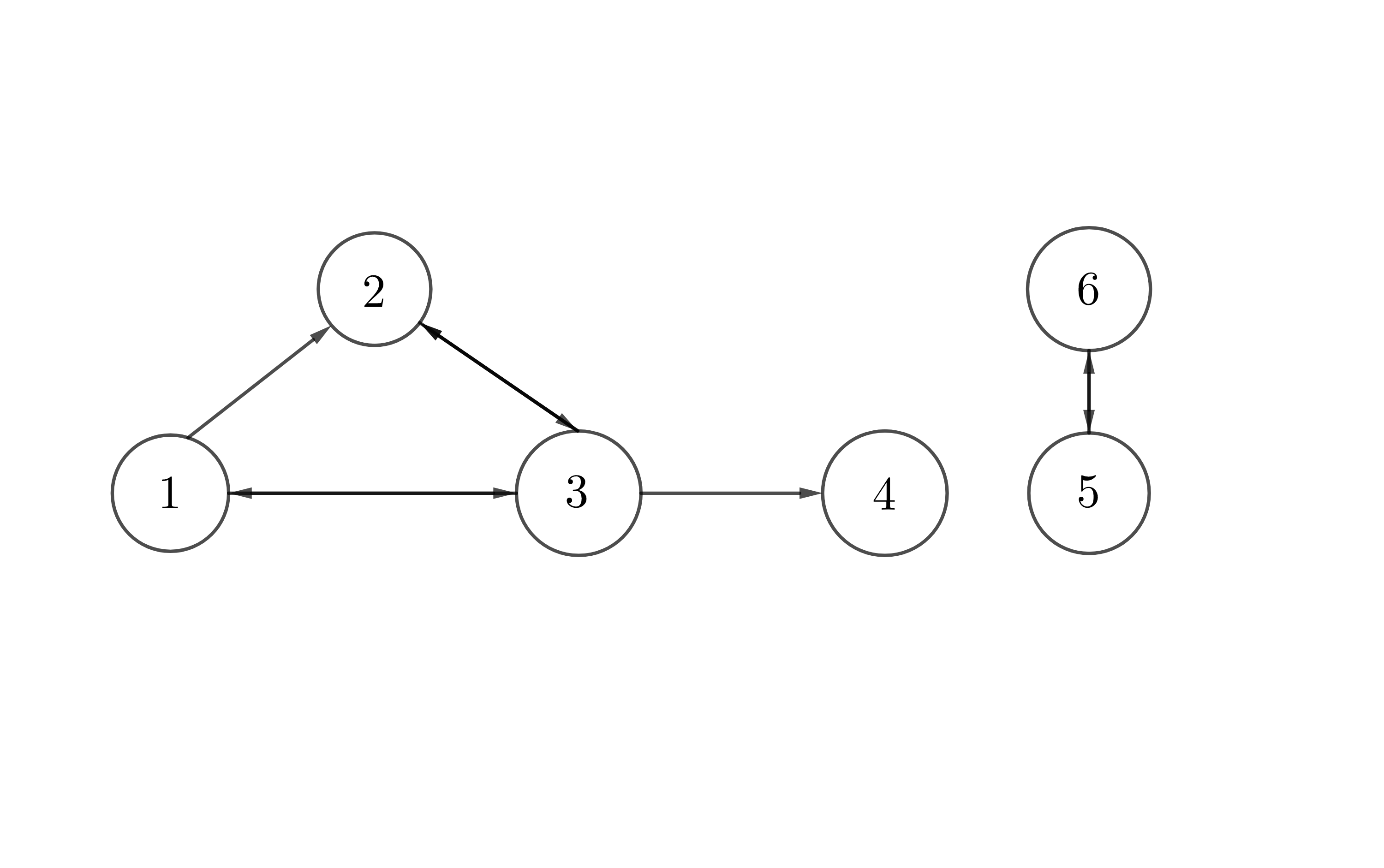 Figure 10.13: Six pages
For a directed network, the edge \(\{\mbox{red},\mbox{green}\}\) does not mean \(\{\mbox{green},\mbox{red}\}\). One has to figure out the valid direction of the relation. One popular directed network model, called PageRank algorithm, was developed by google for matching the desired web pages in a search engine. Suppose a web of six pages represented as in figure 10.13 with pages as vertices and links from one page to another (arrows) as directed edges. To rank the importance of a page, we could count the incoming links (called backlinks) of each page and then rank pages according to the counting score. Let the score for page \(i\) be \(x_{i}\). One can define \(x_{i}\) as \(x_{i}=\sum_{j\sim i}x_{j}/\mbox{deg}(j)\) where \(j\sim i\) and \(\mbox{deg}(j)\) measures the total number of outgoing links on the page \(j\).178 The equation says each page divides its one unit of influence among all pages to which it links, so that no page has more influence to distribute than any other. From figure 10.13, we have the adjacency matrix as well as the matrix for the scores \[\mathbf{A}=\left[\begin{array}{cccccc} 0 & 0 & 1 & 0 & 0 & 0\\ 1 & 0 & 1 & 0 & 0 & 0\\ 1 & 1 & 0 & 0 & 0 & 0\\ 0 & 0 & 1 & 0 & 0 & 0\\ 0 & 0 & 0 & 0 & 0 & 1\\ 0 & 0 & 0 & 0 & 1 & 0 \end{array}\right],\quad\mathbf{P}=\left[\begin{array}{cccccc} 0 & 0 & 1/3 & 0 & 0 & 0\\ 1/2 & 0 & 1/3 & 0 & 0 & 0\\ 1/2 & 1 & 0 & 0 & 0 & 0\\ 0 & 0 & 1/3 & 0 & 0 & 0\\ 0 & 0 & 0 & 0 & 0 & 1\\ 0 & 0 & 0 & 0 & 1 & 0 \end{array}\right]\] where \(\mathbf{P}\) is to divide each column \(j\) of \(\mathbf{A}\) by the degree of this vertex \(j\). The system of the page scores is given by \[\mathbf{x}=\mathbf{P}\mathbf{x}\] which tells us is that the desired ranking vector \(\mathbf{x}\) is really a stationary vector for the matrix \(\mathbf{P}\). Since \(\mathbf{x}\) appears as the input and the output of this linear system, the system is referred to a linear simultaneous system.
The linear simultaneous system is a fundamental tool for modeling input-output relations. Let’s assume that in an economy with \(n\) different industrial sectors, the total production output of sector \(i\) is \(x_{i}\) for \(i=1,\dots,n\). The output of each sector can flow to other sectors for supporting the production or it can flow to the consumers. Let the demand for sector \(i\) be \(d_{i}\). Let the input-output matrix \(\mathbf{A}\) characterize the flows between the sectors. For example, the output \(x_{j}\) in the sector \(j\) requires \(a_{ij}x_{j}\) unit input from the sector \(i\). The full expression of this economy becomes \[\mathbf{x}=\mathbf{A}\mathbf{x}+\mathbf{d}\] which means that the total production of each sector matches the demand of this sector plus the total amount required to support production in this sector. The model is known as (Leontief’s) input-output model.
10.5 Miscellaneous: Mythology and Symbolism
As we have seen that the additions of vectors and matrices are somehow different from the additions of numbers. The “+” sign attached to these addition is merely a symbol. When we endow this symbol to the general meaning (the four axioms), this symbol is equipped with new significance. And the new significance does include the specific meaning of the addition of integers.
Symbolization belongs to abstraction - a genral reference to the realm of reality from which the form (in a philosophical sense) is abstracted, a reflection of the laws of that realm, a “logical picture” into which all instances must fit.
Symbols have their roles in religious rituals and in scientific explorations. The fundamental perspective of most religions is the notion of embodying a timeless truth that was derived either from a divine source or from some insight into an unchanging reality. It may be a challenge for religions to admit that something absolutely basic to the world can be changed as the evolutionary meanings of symbols. However, in response to the transitions (and perhaps the associated threats), religious did use symbols to expand their explainable and inferential power. Ancient Chinese founded their religious or eastern philosophical system by divinatory symbols representing the changes of nature. Five elements (earth, metal, water, wood and fire), for example, was a skeleton in the Chinese belief. With such belief, the phenomena in astrology, medicine, military strategy, etc., were successively interpreted on the basis of these five symbols. Gradually, the five elements based interpretations reinforce Chinese belief of the world as such.
By symbols, one can transfer experiences that no other medium can adequately express. Aesthetic attraction and mysterious fear are probably the first manifestations of the symbolization in which people perceived some peculiar tendencies of visualizing the reality, and by which they were able to concretize some abstract concepts and projected them into the reality. When there were no clear casuality among the features, people were intended to attach some distant features to the existing symbolic meanings, and the meanings later would react upon the people. It creates a closed loop to control the humans cognitions towards the unknown casuality and gives the initial consciousness of the scientific reasoning.
Although symbols have rich content and hidden natures, they are vague and lack of definitive explainations.179 Can the indirect ways express more absolute truths? Can abstract symbols compress more information than concrete characters? Thinking these questions systematically may stimulate your spiritual resonance of symbolization. The evolutionary paths of symbolization is diverse. When Chinese attached their worldview firmly with the fixed symbolic system made of five elements and eight trigrams, and completed a self-consistent reasoning logic as “theory of everything;” on the contrary, the symbolization in western world was able to detach from the preconceived areas, explored and evolved into a much deeper field, and created a more abstract vision of the world. From late 19th century to early 20th century, the core period of the second industrial revolution as well as the period of reflection and self-examination with the rise of communism and social Darwinism on the eve of the WWI, the symbolism declared to abandon the direct reproduction of reality, and to focus on the multifaceted synthesis of the phenomena.180 In arts and literature, symbolism foucses on the brimming situations with emotional content and expressive energy. One representative work of this style can be found in Les Fleurs du mal, a volume of poetry written by Charles Baudelaire. The movement somehow successfully implied various thoughts through polysemous symbols.
Miscellaneous
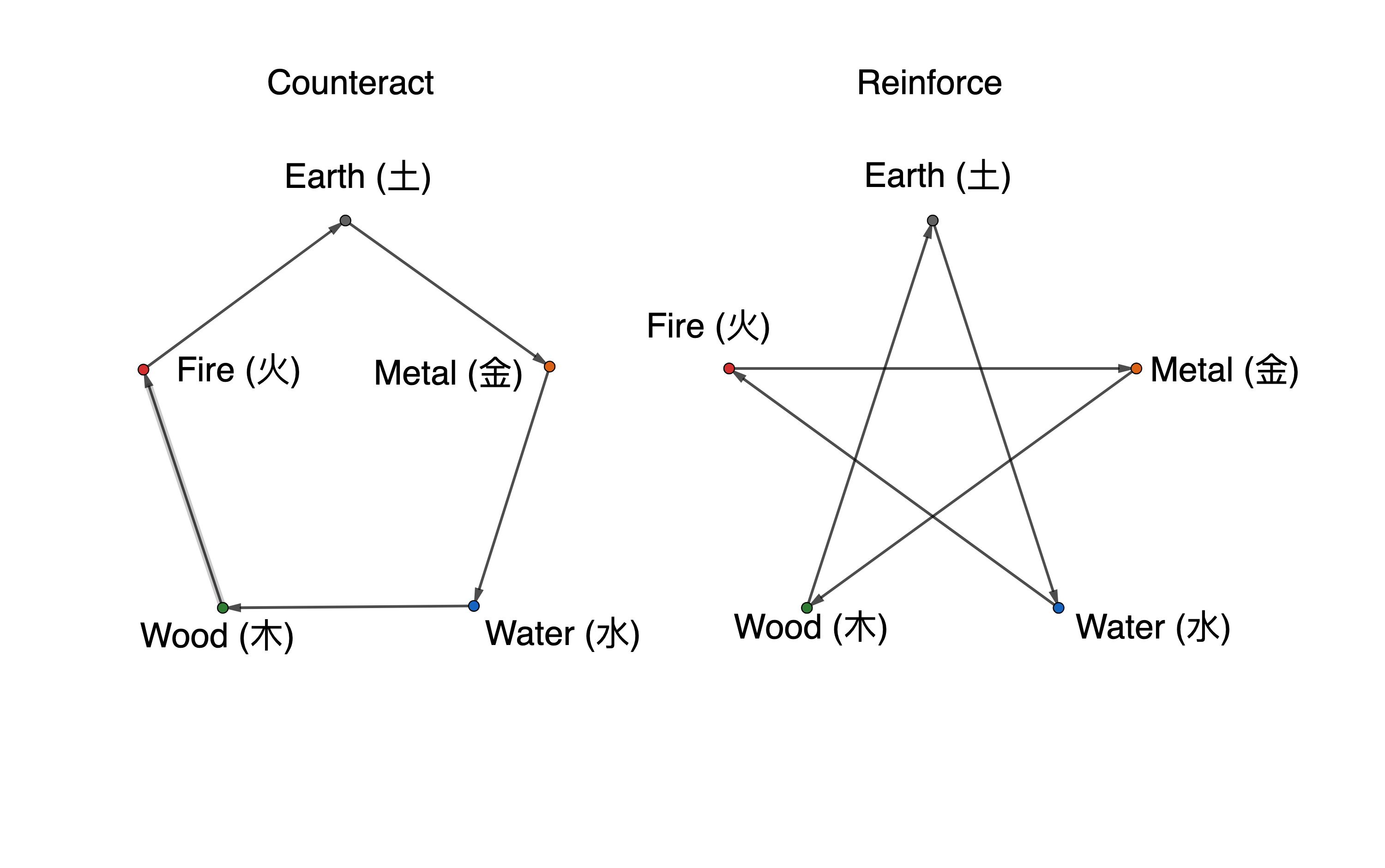 Figure 10.14: Five elements in Daoism
Page built: 2023-01-03