12 Eigenvalues and Eigenvectors
If we could express the change of the milieu in a computational form, then the matrix computation of \(\mathbf{A}\mathbf{x}\) could describe the generation and the transformation of such milieu. The input \(\mathbf{x}\) could be stimulus and cause, and the output \(\mathbf{A}\mathbf{x}\) could be reaction and effect. In other words, if the information of the current world were stored in a (huge) vector \(\mathbf{x}\) in an \(n\)-dimensional field, then the (linear) dynamics of this world were conducted by an \(n\times n\) matrix \(\mathbf{A}\).
Figure 11.2 shows the transformations of vectors in a 2-dimensional vector space. We can see that those directions and orientations (in purple and red lines) remain consistent with the transformation. By stretching and compressing the directional arrows, we can scale their magnitudes (scalars) under which the transformation looks invariant. Generally speaking, this kind of invariance exists for any \(n\times n\) matrix \(\mathbf{A}\), and it is analyzable under the framework of eigenvalues and eigenvectors.216 For non-square \(m\times n\) matrices \(\mathbf{A}\), we can use an alternative framework of singular values and singular vectors. Roughly speaking, the singular values are the positive square roots of the nonzero eigenvalues of the corresponding matrix \(\mathbf{A}^{\top}\mathbf{A}\). The corresponding eigenvectors are called the singular vectors. Eigenvalues and eigenvectors can be mathematically defined as sets of invariants within processes of transformations. As matrixs can store all sorts of data information, eigenvalues and eigenvectors can in turn represent the corresponding “script lines” with clearly directional “stages”.
Perhaps the infinitely embodying milieu as computations of matrices makes the symbolization impossible. But as a conceptual ideal, the embodiment of eigenvalues and eigenvectors provide a way to recognize two seperated channels of forming one’s perception, the (concrete) material channel and the (imginary) spiritual one. The logic of using eigenvalues and eigenvectors - that is, the identification, the trace and maybe the selection of its various structural invariants - can reconfigure the relation of the input and output channels of the computation. Physical and metaphysical forces from the aspects in the ontology and the epistemology, form these complemenary channels in milieux.
As long as a secular transformation, such as a trade or a production, can be expressed in an input-output matrix form, the eigenvalue and the eigenvector can reconfigure the form as an epistemological and ontological emergence. Maybe I can call this process the valuation. The valuation here is defined as the emergence of quantitative “being” that attaches to the transformation, and remains invariant when the structure of the transformation unchanges.
12.1 Determinants, Characteristic Polynomials, and Complex Numbers
The detective novel often depicts a fragmentary plot to drive the readers in a complete daze. When the readers were attracted by various bizarre and outrageous transforming scenes, the author, quite likely, had buried the solution clue in some unaltered remainders.
For mathematical transformations, in passing from one equation to the other, what was left unchanged is called an invariant. We will explore the invariant properties of the linear transformations through the determinant. A determinant of a square matrix \(\mathbf{A}\), denoted by \(\mbox{det}(\mathbf{A})\), is a function mapping \(\mathbf{A}\) to a real number. This real number contains the information about the product of all pivots of the echelon form of \(\mathbf{A}\).
Consider a \(2\times2\) matrix \[\mathbf{A}=\left[\begin{array}{cc} a_{11} & a_{12}\\ a_{21} & a_{22} \end{array}\right].\] The pivots of \(\mathbf{A}\) are \(a_{11}\) and \(a_{22}-(a_{21}/a_{11})a_{12}\). The product of these pivots is \(a_{11}(a_{22}-(a_{21}/a_{11})a_{12})=a_{11}a_{22}-a_{21}a_{12}\). The determinant is sometimes written with a single straight line as left and right brackets. So we would write the above result as \[\mbox{det}(\mathbf{A})=\left|\begin{array}{cc} a_{11} & a_{12}\\ a_{21} & a_{22} \end{array}\right|=a_{11}a_{22}-a_{12}a_{21}.\]
If we think of \(\mathbf{A}\) as two row vectors in the plane, i.e. \(\mathbf{A}=[\mathbf{a}_{1},\mathbf{a}_{2}]^{\top}\), then the determinant is the (signed) area of the parallelogram spanned by \(\mathbf{a}_{1}\) and \(\mathbf{a}_{2}\). The sign of the determinant is positive (negative) if the two vectors are positively (negatively) oriented. Figure 12.1 shows a parallelogram spanned by \(\mathbf{z}=[5,1]\) and \(\mathbf{u}=[-1,3]\).
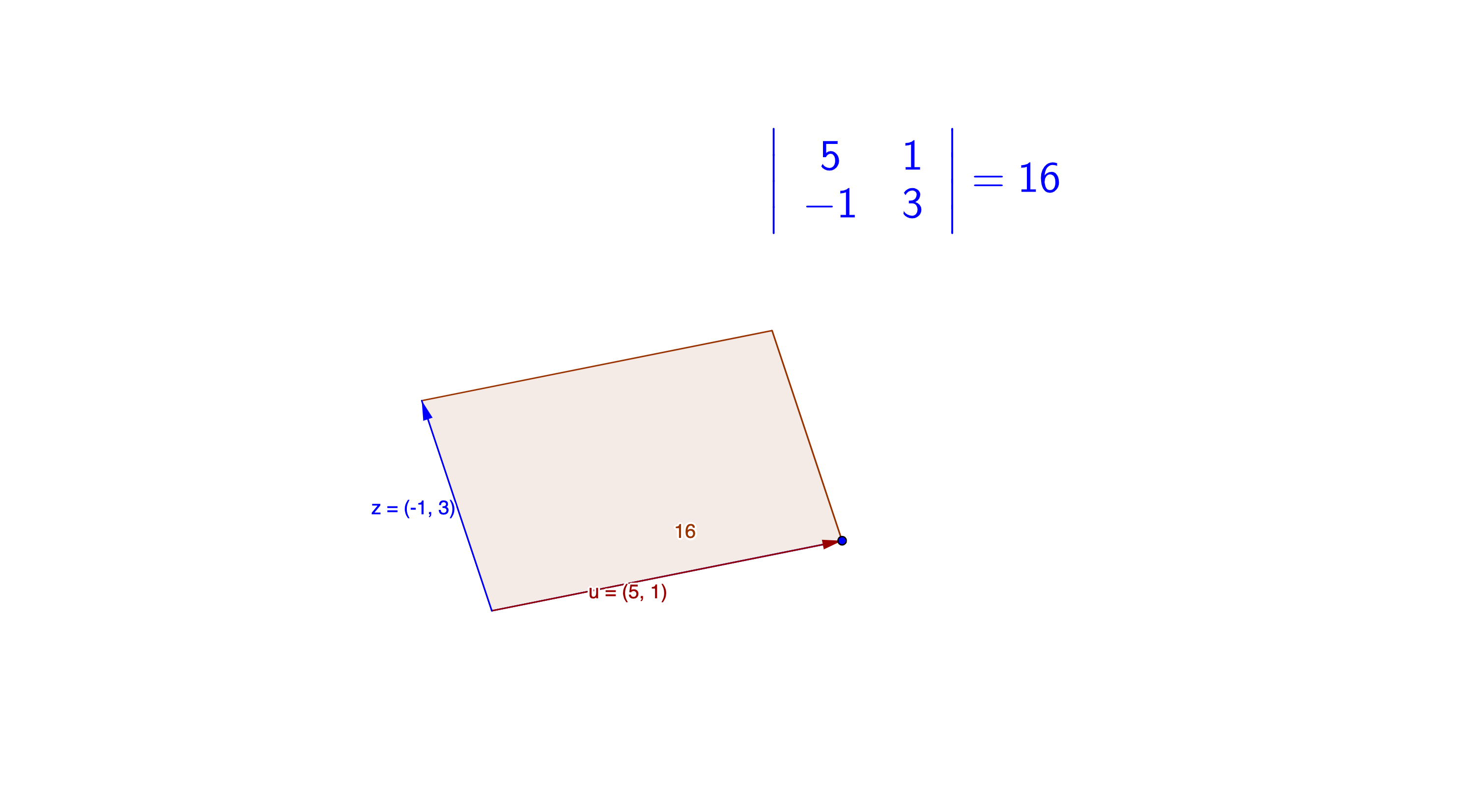 Figure 12.1: Determinant in a parallelogram
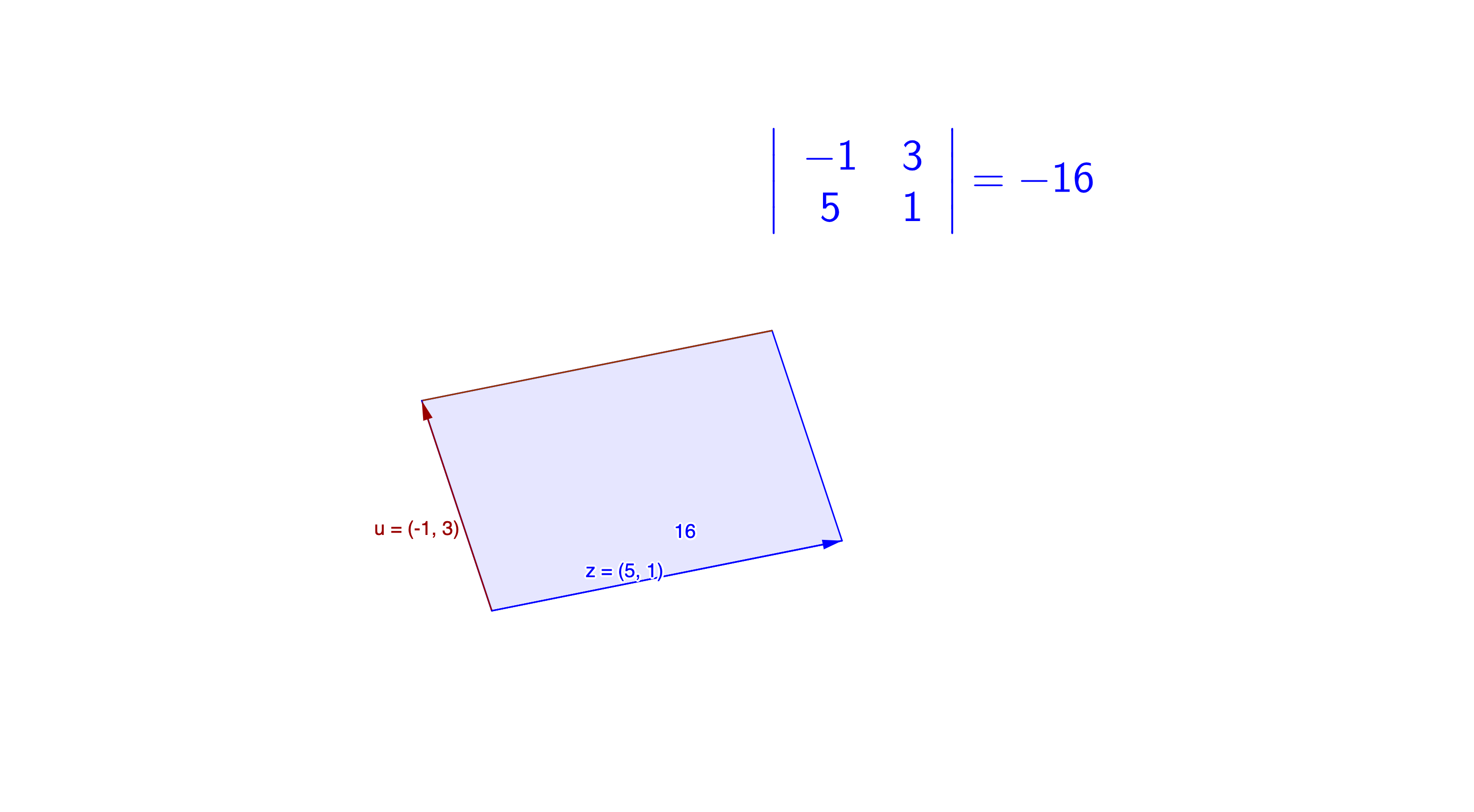 Figure 12.1: Determinant in a parallelogram
For an invertible \(n\times n\) matrix \(\mathbf{A}\), its echelon form says that all pivots are non-zero217 As the statement in section 11.2, the determinant also relates the invertibility of \(\mathbf{A}\). A zero determinant induces a non-invertible/singular square matrix., so is the product of all pivots, namely \(\mbox{det}(\mathbf{A})\neq 0\). Geometrically, the absolute value of \(\mbox{det}(\mathbf{A})\) is equal to the volume of the \(n\)-dimensional parallelepiped, where the \(n\)-dimensional parallelepiped spanned by the column or row vectors of \(\mathbf{A}\).218 The determinant of \(\mathbf{A}\) is positive or negative according to whether the linear mapping \(\mathbf{A}\mathbf{x}\) preserves or reverses the orientation of the \(n\)-dimensional \(\mathbf{x}\). The absolute value of the determinant can be thought of as a measure of how much multiplication by the matrix expands or contracts the space of \(\mathbf{x}\). If the determinant is \(0\), then space is contracted completely along at least one dimension, causing it to lose all of its volume. If the determinant is \(1\), then the transformation preserves volume.
Here is a list of some properties (facts) of the determinant of a square \(n\times n\) matrix.
\(\mbox{det}(\mathbf{I})=1\).
\(\mbox{det}(\mathbf{A})=0\), if the matrix \(\mathbf{A}\) is singular or non-invertible.
Swapping two vectors of \(\mathbf{A}\) changes the sign of \(\mbox{det}(\mathbf{A})\). In other words, \(\mbox{det}(\mathbf{E}_{ij}\mathbf{A})=-\mbox{det}(\mathbf{A})\) where \(\mathbf{E}_{ij}\) is the permutation elementary matrix.
Scaling a row or a column of \(\mathcal{A}\) scales the determinant. In other words, \(\mbox{det}(\mathbf{E}_{i}(c)\mathbf{A})=c \times \mbox{det}(\mathbf{A})\) where \(\mathbf{E}_{i}(c)\) is the scaling elementary matrix.
For the replacement elementary matrix, \(\mbox{det}(\mathbf{E}_{ij}(s)\mathbf{A})=\mbox{det}(\mathbf{A})\).
Note that the determinants of triangular matrices and diagonal matrices are exactly the product of the diagonal entries in those matrices. Fact 1) comes directly from the product of ones on the diagonal of \(\mathbf{I}\). Fact 2) comes from the definition. Figure 12.1 gives an example of 3). For 4), figure 12.2 shows how the scaling transformation changes the determinant (the area of the parallelogram). For fact 5), figure 11.1 shows that in the Gaussian elimination procedures, forming the echelon form do not affect the volume. In other words, the replacement elementary matrices simply rotate the intersections of the parallelepiped, and preserve the volume.
 Figure 12.2: Determinants of the scaling transformations
Another definition of the determinant
With the previous five results, it is possible to derive further properties:
\(\mbox{det}(\mathbf{A}\mathbf{B})=\mbox{det}(\mathbf{A})\mbox{det}(\mathbf{B})\).
\(\mbox{det}(\mathbf{A}+\mathbf{B})=\mbox{det}(\mathbf{A})+\mbox{det}(\mathbf{B})\).
\(\mbox{det}\mathbf{A}^{\top}=\mbox{det}\mathbf{A}\).
\(\mbox{det}(\mathbf{A}^{-1})=\frac{1}{\mbox{det}(\mathbf{A})}\).
Sketch of the proof
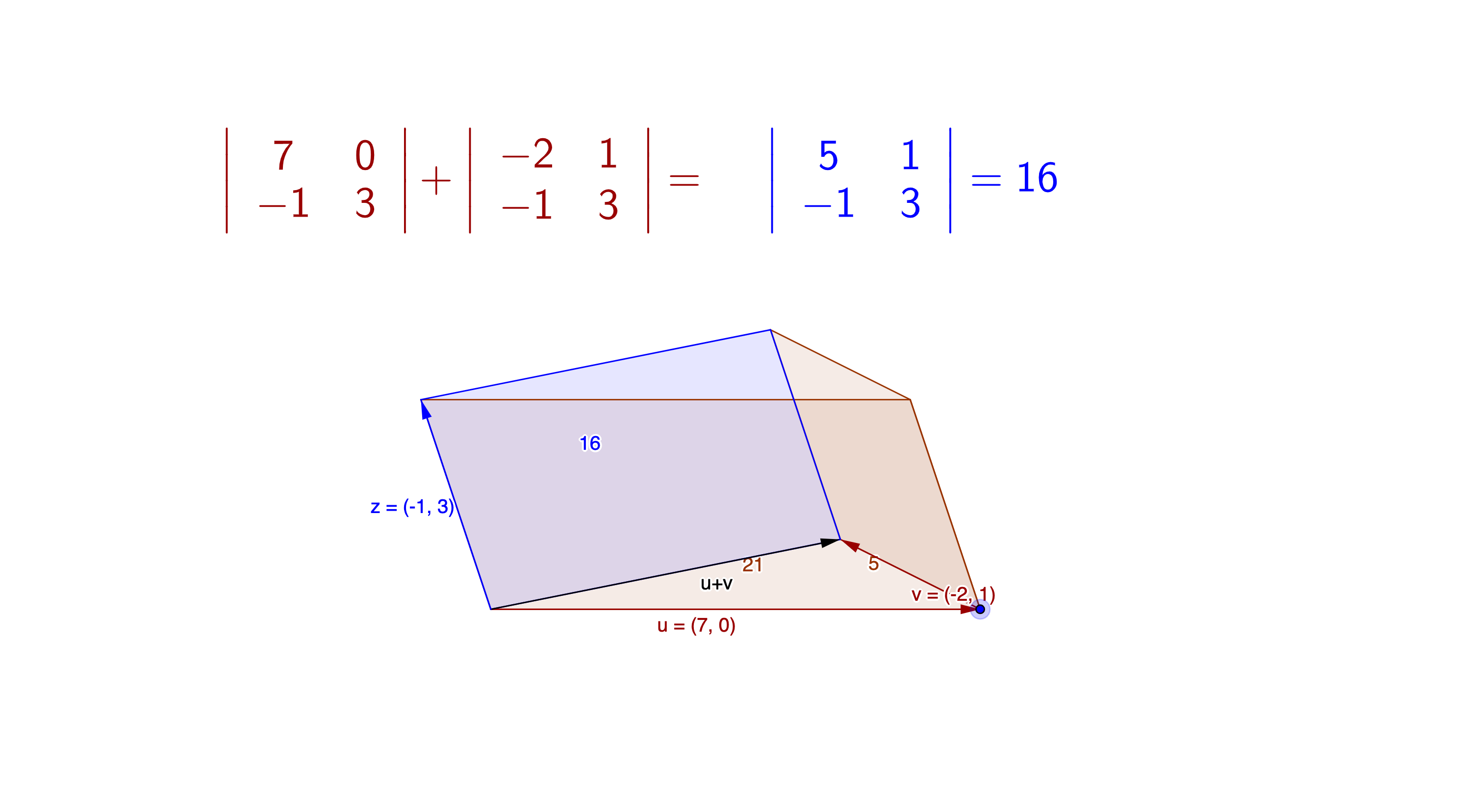 Figure 12.3: Determinant of the matrix addition
To see the use of determinant, let’s return to the fixed point problem in the matrix form \(\mathbf{A}\mathbf{x}=\mathbf{x}\) where the transformation is invariant around the solution \(\mathbf{x}^{*}\). Suppose \(\mathbf{A}\) is an \(n\times n\) invertible matrix, we will see that the existence of \(\mathbf{x}^{*}\) can be determinated by the determinant of \(\mathbf{A}\).
Notice that the fixed point problem can be presented as \(0=\mathbf{x}-\mathbf{A}\mathbf{x}\) or \[0=(\mathbf{I}-\mathbf{A})\mathbf{x}.\] The statement 4) in section 11.2 says that for an invertible matrix \(\mathbf{I}-\mathbf{A}\), \((\mathbf{I}-\mathbf{A})\mathbf{x}=0\) has a unique solution \(\mathbf{x}^{*}=0\). This statement implies that if we are looking for a non-zero solution of \(\mathbf{x}^{*}\), we should expect that \(\mathbf{(\mathbf{I}-\mathbf{A})}\) to be singular or non-invertible, namely \(\mbox{det}(\mathbf{I}-\mathbf{A})=0\). In this way, the existence of a non-zero fixed point solution \(\mathbf{x}^{*}\) is equivalent to a zero determinant of \(\mathbf{I}-\mathbf{A}\).
The linear transformation of the fixed point problem \(\mathbf{A}\mathbf{x}^{*}=1\times \mathbf{x}^{*}\) preserve the invariant \(n\)-vector \(\mathbf{x}^{*}\). We can call the vector \(\mathbf{x}^{*}\) the eigenvector of \(\mathbf{A}\) with eigenvalue \(1\). The formal definition of eigenvector and eigenvalue is given by the characteristic polynomial.
- Eigenvector, eigenvalue, characteristic polynomial : Consider an \(n\times n\) matrix \(\mathbf{A}\in\mathbb{F}^{n\times n}\), where the field \(\mathbb{F}\) can be \(\mathbb{C}\) or \(\mathbb{R}\). The eigenvalues of \(\mathbf{A}\) are the \(n\) roots, \(\Lambda=\{\lambda_{1},\dots,\lambda_{n}\}\), of its characteristic polynomial \[\mbox{det}(\lambda\mathbf{I}-\mathbf{A}).\] The set of these roots is called the spectrum of \(\mathbf{A}\), and it can also be written as\[\mathcal{S}=\{\lambda \in {\mathbb{C}} \,:\mbox{det}(\lambda\mathbf{I}-\mathbf{A})=0\}.\] For any \(\lambda\in\mathcal{S}\), the non-zero vector \(\mathbf{v}\in\mathbb{C}^{n}\) that satisfies \(\mathbf{A}\mathbf{v}=\lambda\mathbf{v}\) is an eigenvector.
The definition says that solving the characteristic polynomial gives us the eigenvalues \(\lambda\). Given the eigenvalues \(\lambda\), the solution of \(\mathbf{A}\mathbf{v}=\lambda\mathbf{v}\) (or as a fixed point problem: \((\mathbf{A}/\lambda)\mathbf{v}=\mathbf{v}\)) gives the corresponding eigenvectors. All the information of the transformation \(\mathbf{A}\mathbf{v}\) is now preserved by \(\lambda \mathbf{v}\). In other words, the information of linear transformations \(\mathbf{A}\) is stored by the pairs \(\lambda\) and \(\mathbf{v}\).
Here are some straightforward properties about the eigenvalues.
- Let \(\lambda\mathbf{I}\) be \(\Lambda\). \(\mbox{det}(\mathbf{A})=\mbox{det}(\Lambda)=\lambda_{1}\lambda_{2}\cdots\lambda_{n}\).
Because \(\mbox{det}(\lambda\mathbf{I}-\mathbf{A})=0\), the determinant fact 7) implies \(\mbox{det}(\lambda\mathbf{I})=\mbox{det}(\mathbf{A})\). Notice that \(\lambda\mathbf{I}=\Lambda\) is a diagonal matrix, so \(\mbox{det}(\Lambda)=\lambda_{1}\lambda_{2}\cdots\lambda_{n}\).
We will consider more examples about eigenvalues and eigenvectors in the following sections. At the moment, we focus on the illumination of invariant property given by the characteristic polynomial and its determinant.219 Our exposition introduced matrices first and determinants later, however the historical order of discovery was the opposite: determinants were known long before matrices. Also, the recognition of an invariant as an quantitative object in its own interest emerged together with the determinants (characteristic polynomials). Perphas, the most familiar invariant for a polynomial is the discriminant \(b^{2}-ac\) from a quadratic form (a bivariate polynomial) \[ax_{2}^{2}+2bx_{1}x_{2}+cx_{2}^{2}.\] The discriminant indicates properties of the roots for this bivariate polynomial regardless the specific values of \(a\), \(b\) and \(c\). One feature about this invariant is that after any linear transformation vector \([x_{1},x_{2}]\), the discriminat \(b^{2}-ac\) still works.
The discriminant of bivariate polynomials illuminates that searching the invariant property may receive more rewards than calculating a specific solution. The solution of the polynomial varies when the polynomial is changed by the structure (coefficients), but the discriminant formula remains unchanged. Moerover, the formula also determines the new solution values. Thus, when we face various systems, it may be more worthy to find the invariant shared by these systems rather than solve each system one by one.
In an economy of \(n\)-sectors, one can model both the supply and the demand system of this economy by polynomials. That is, if we have one system, say the supply system, of \(n\)-factors (variables), and we expect that there is another corresponding but different system of the same factors.220 The factors in different sides may require different quantities, so these two system cannot have the same form. Suppose the factor in the demand side (output) has to be transformed from the supply side (input). An invariant of this economy means that the transformation for the factors can equate the supply system with the demand one for all \(n\)-sectors. We use a quantitative model to illustrate how to identify the invariant.
Invariants in the multivariate polynomial system
So far, we only saw the univariate polynomial. A more general multivariate polynomial system in the vector space \(\mathcal{V}\subset\mathbb{R}^n\) allows arbitrary \(n\)-unknowns, namely an \(n\)-length variable vector \(\mathbf{x}=[x_1,\dots,x_n]\). Each term of such a polynomial is called the monomial221 One widely used function of modelling productions and utilities is the Cobb-Douglas function. Its standard form is \[y = c(x_1)^{\alpha_1}(x_2)^{\alpha_2}\] where \(y\) is the output of the function and \(\mathbf{x}\) can be interpreted as the production factors, such as labor and capital, or it can be a consumption plan of two different goods. \[x_{1}^{\alpha_{1}}x_{2}^{\alpha_{2}}\cdots x_{n}^{\alpha_{n}},\quad \mbox{ where } \mathbf{x}=[x_{1},\cdots,x_{n}]\in\mathcal{V}, \,\, \alpha_{i}\in\mathbb{N}^{+}.\] Here \(\alpha_{i}\in\mathbb{N}^{+}\) means these power indexes are positive integers. We consider a system of multivariate polynomials with \(n\)-unknowns and with the total order of the monomial less than \(n\): \[\mathcal{P}_{n}(\mathcal{V})=\left\{ \left.f(\mathbf{x})=\sum_{i}c_{i}x_{1}^{\alpha_{i,1}}x_{2}^{\alpha_{i.2}}\cdots x_{n}^{\alpha_{i,n}}\right|\,\mathbf{x}\in\mathcal{V},\quad\alpha_{i,1}+\cdots+\alpha_{i,n}\leq n,\:\alpha_{i,j},\:\alpha_{i,j}\in\mathbb{N}^{+} \right\} \]
In this general \(n\)-th order multivariate polynomial system, the invariants under the linear transformation of \(\mathbf{x}\) relate to the determinants of the transformation. Suppose the vector \(\mathbf{y}\) is linearly transformed from the vector \(\mathbf{x}\) by \(\mathbf{A}\), such that \(\mathbf{y}=\mathbf{A}\mathbf{x}\) with \(\mathbf{A}=[a_{ij}]_{n\times n}\). Assume that the supply function \(p(\mathbf{x})\), and the demand function \(q(\mathbf{y})\in\mathcal{P}_{n}(\mathcal{V})\) are two multivariate polynomials with \(n\) unknown quantities in \(n\)-sectors.
If there is an invariant in \(p(\mathbf{x})\) and \(q(\mathbf{y})\) by making \(p(\mathbf{x})=q(\mathbf{y})\), then any infinitesimal changes of \(p(\mathbf{x})\) and \(q(\mathbf{x})\) should not violate the equality. So we expect that after taking the partial derivatives the equality still holds: \[ \begin{align*} \frac{\partial p}{\partial y_{1}}\frac{\partial y_{1}}{\partial x_{1}}+\cdots+&\frac{\partial p}{\partial y_{n}}\frac{\partial y_{n}}{\partial x_{1}} =\frac{\partial q}{\partial x_{1}},\\ \frac{\partial p}{\partial y_{1}}\frac{\partial y_{1}}{\partial x_{2}}+\cdots+&\frac{\partial p}{\partial y_{n}}\frac{\partial y_{n}}{\partial x_{2}} =\frac{\partial q}{\partial x_{2}},\\ \vdots & \qquad \quad \vdots \\ \frac{\partial p}{\partial y_{1}}\frac{\partial y_{1}}{\partial x_{1}}+\cdots+&\frac{\partial p}{\partial y_{n}}\frac{\partial y_{n}}{\partial x_{n}} =\frac{\partial q}{\partial x_{n}}. \end{align*} \]
Because \(\mathbf{y}=\mathbf{A}\mathbf{x}\) or \[ \begin{align*} a_{11}x_{1}+\cdots+a_{1n}x_{n} &=y_{1},\\ a_{21}x_{1}+\cdots+a_{2n}x_{n} &=y_{2},\\ \vdots\qquad \quad & \vdots \\ a_{m1}x_{1}+\cdots+a_{mn}x_{n} &=y_{n}, \end{align*} \]
we can see that \(\partial y_{i}/\partial x_{j}=a_{ij}\). So the above system can be expressed as \(\mathbf{A}\nabla p=\nabla q\), where \(\nabla p=[\partial p/\partial y_{i}]_{n\times1}\) and \(\nabla q=[\partial q/\partial x_{i}]_{n\times1}\) are the gradient vectors. If the infinitesimal changes of \(q(\mathbf{x})\), namely \(\nabla q\), is zero, then we expect \(\nabla p\) to be zero. In other words, the linear system \(\mathbf{A}\nabla p=0\) has the solution \(\nabla p=0\) if and only if \(\mbox{det}(\mathbf{A})\neq0\). (Statement 4 in section 11.2.)
Thus the condition \(\mbox{det}(\mathbf{A})\neq0\) is to ensure the existence of the invariant in this system. Then Gaussian elimination can reduce the linear system \(\mathbf{A}\nabla p= 0\) to an expression of the invariant.
The idea of this method, an algebra perspective of bridging the invariance and the determinant of the partially differentiable transformation (the coefficient matrix \(\mathbf{A}\)), was first proposed by Boole (1841).222 Some British mathematicians even said the study of partial differential equations was initiated by the exploration of the invariant. I am not sure how proper the statement is, but indeed many early efforts of looking for an invariant were on the path of searching for an equivalent solution of some system of partial differential equations.
Invariants of the discriminant in the bivariate polynomial
Another important implication from the definition of characteristic polynomial is that the eigenvalues, as the solutions of the characteristic polynomial, belong to the complex number field \(\mathbb{C}\). This is the case for both the real valued and the complex valued matrix \(\mathbf{A}\) in \(\mathbf{A}\mathbf{v}=\lambda\mathbf{v}\). This implication comes from the fundamental theorem of algebra.
- Fundamental theorem of algebra: For a \(n\)-th order polynomial \(f(x)\)=\(a_{0}+a_{1}x+\cdots a_{n}x^{n}\) with real (or complex) number coefficients \(a_{0},\dots,a_{n}\), the polynomial equation \(f(x)=0\) always has a solution in the complex field \(\mathbb{C}\).
 Figure 12.4: Fundamental theorem of algebra
The proof of theorem is beyond our concern. But figure 12.4 gives a rough idea why the theorem works. Suppose we restrict the domain of a polynomial \(f(z)\) to a circle \(|z|\leq r\) where any \(z\in\mathbb{C}\) is a complex number. Then by enlarging the radius \(r\) of the circle, the image (cross-hatching area) \(\{f(z): \, |z|\leq r \}\) will sooner or later cover the zero origin, namely \(f(z)=0\) has a solution \(z^*\) where \(|z^*|\leq r\). This may not be the case if we restrict the domain to a real line of the complex plane.
By the theorem, we can deduce that the complex number system is in the sense of a complete system such that we can solve any polynomial equation in it. The highest degree of a polynomial gives you the highest possible number of distinct complex roots for the polynomial.
Due to the importance of complex number system, hereby we review some basic concepts, and provide some interpretations about the complex number system \[\mathbb{C}=\{a+\mbox{i}b:\, a,b\in\mathbb{R}\}.\] For a complex number \(z\in\mathbb{C}\), \(z=a+\mbox{i}b\) is the standard form. The real part of \(z\) is written as \(\mbox{Re}(z)=a\), and the imaginary part is written as \(\mbox{Im}(z)=b\). The imaginary number \(\mbox{i}\) satisfies the algebraic identity \(\mbox{i}^{2}=-1\). The complex conjugate of \(z\), having the same real part of \(z\) but the opposite imaginary part, is defined as \(\bar{z}=a-\mbox{i}b\). Two complex numbers are equal precisely when they have the same real part and the same imaginary part.
One can also consider that the complex numbers as ordered pairs of real numbers satisfying the law of complex arithmetic. As complex numbers behave like ordered pairs of real numbers, they can be identified with points in the plane. Real numbers go along the \(x\)-axis, and imaginary numbers are on the \(y\)-axis. This gives the complex plane. Arithmetic of addition and subtraction in \(\mathbb{C}\) is carried out like adding and subtracting vectors in \(\mathbb{R}^{2}\). Arithmetic of multiplication in \(\mathbb{C}\) and the norm, however, are different those of vectors in \(\mathbb{R}^{2}\).223 The law of complex arithmetic includes addition \((a+\mbox{i}b)+(c+\mbox{i}d)=(a+c)+(b+d)\mbox{i}\), multiplication \((a+\mbox{i}b)(c+\mbox{i}d)=(ac-bd)+(ad+bc)\mbox{i}\), absolute value (or square root of the norm) \(|a+\mbox{i}b|= \sqrt{a^{2}+b^{2}}=\sqrt{(a+\mbox{i}b)(a-\mbox{i}b)}\).
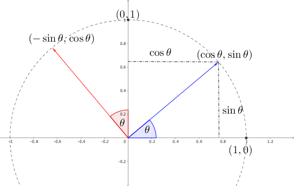 Figure 12.5: Rotation of complex numbers
For the multiplication of complex numbers, it may be more straightforward to consider under the polar coordinate. For a complex number \(z=a+\mbox{i}b\) with \(|z|=r\), its polar form is \(z=r\mbox{e}^{\mbox{i}\theta}\) or \(z=r\cos\theta+\mbox{i}r\sin\theta\).224 Euler identity showes that the exponent of an imaginary number power can be turned into the sines and cosines of trigonometry via \[\mbox{e}^{\mbox{i}\pi}=-1.\] The identity comes from the Euler formula \(\mbox{e}^{\mbox{i}\theta}=\cos\theta+\mbox{i}\sin\theta\). Thus, any point on a plane comes with the polar coordinate pair \((r\cos\theta,r\sin\theta)\). where the real number \(r\) represents the absolute value of \(z\), namely \(r=|z|=\sqrt{a^{2}+b^{2}}\), and \(\theta\) represents the angle. By using the property of the exponential function, the polar form can easily tell us that \(z^{n}=r^{n}\mbox{e}^{\mbox{i}n\theta}=r^{n}(\cos n\theta+\mbox{i}\sin n\theta)\), where the absolute value \(|z^{n}|=r^{n}\) and the angle is \(n\times \theta\). Also, for the complex multiplication of \(z_1=r_1\mbox{e}^{\mbox{i}\theta_1}\) and \(z_2=r_2\mbox{e}^{\mbox{i}\theta_2}\), it is all about rescaling the absolute value to \(r_1\times r_2\) and rotating the angle to \(\theta_1+\theta_2\).
The complex multiplication on a unit circle also relates to a linear transformation. From figure 12.5, we can see that a rotation of the plane on \(\mathbb{R}^{2}\) around the origin through angle \(\theta\) is a linear transformation that sends the basis vectors \([1,0]\) and \([0,1]\) to \([\cos\theta,\sin\theta]\) and \([-\sin\theta,\cos\theta]\), respectively. Let’s denote this transofrmation \(\mathbf{T}_{\theta}\) by \[\mathbf{T}_{\theta}\left(x\left[\begin{array}{c} 1\\ 0 \end{array}\right]+y\left[\begin{array}{c} 0\\ 1 \end{array}\right]\right)=\left[\begin{array}{c} x\cos\theta-y\sin\theta\\ x\sin\theta+y\cos\theta \end{array}\right].\] In fact, this linear transformation can be represented by the matrix \[\mathbf{T}_{\theta}=\left[\begin{array}{cc} \cos\theta & -\sin\theta\\ \sin\theta & \cos\theta \end{array}\right].\] We call \(\mathbf{T}_{\theta}\) the rotation matrix with the angle \(\theta\). Notice that for an arbitrary point \((x,y)\) on the complex plane, the rotation of \(\theta\) angle simply says \[(\cos\theta+\mbox{i}\sin\theta)(x+\mbox{i}y)=x\cos\theta-y\sin\theta+\mbox{i}(x\sin\theta+y\cos\theta).\] That is, each rotation \(\mathbf{T}_{\theta}\) in \(\mathbb{R}^{2}\) can represent the complex number \(\cos\theta+\mbox{i}\sin\theta\).
By decomposing the rotation matrix \[\mathbf{T}_{\theta}=\cos\theta\underset{\mathbf{B}_{1}}{\underbrace{\left[\begin{array}{cc} 1 & 0\\ 0 & 1 \end{array}\right]}}+\sin\theta\underset{\mathbf{B}_{2}}{\underbrace{\left[\begin{array}{cc} 0 & -1\\ 1 & 0 \end{array}\right]}},\] we represent the rotation by the matrices \(\mathbf{B}_1\) and \(\mathbf{B}_2\). One can verify that these two matrices behave exactly the same as the numbers \(1\) (\(\mathbf{B}_1=\mathbf{I}\)) and \(\mbox{i}\) (\(\mathbf{B}_2 \mathbf{B}_2= - \mathbf{I}\)). In fact, any \[\left[\begin{array}{cc} a & -b\\ b & a \end{array}\right]=a\left[\begin{array}{cc} 1 & 0\\ 0 & 1 \end{array}\right]+b\left[\begin{array}{cc} 0 & -1\\ 1 & 0 \end{array}\right],\; a,b\in\mathbb{R}\] behaves exactly the same as the complex number \(a+\mbox{i}b\) under addition and multiplication. In other words, all complex numbers can be represented by these \(2\times2\) real matrices \(a\mathbf{B}_{1}+b\mathbf{B}_{2}\).
The determinant of real matrices \(a\mathbf{B}_{1}+b\mathbf{B}_{2}\) corresponds to the squared norm (squared absolute value) \[\mbox{det}(a\mathbf{B}_{1}+b\mathbf{B}_{2})=|a+\mbox{i}b|^{2}=a^{2}+b^{2}.\] Thus, the multiplicative property of \(|z_{1}z_{2}|=|z_{1}||z_{2}|\) for \(z_{1},z_{2}\in\mathbb{C}\) can be deduced by the multiplicative property of determinants (fact 6).225 The inverse \(z^{-1}=(a-\mbox{i}b)/(a^{2}+b^{2})\) corresponds to the inverse matrix \[\left[\begin{array}{cc} a & -b\\ b & a \end{array}\right]^{-1}=\frac{1}{a^{2}+b^{2}}\left[\begin{array}{cc} a & b\\ -b & a \end{array}\right].\]
As we have seen the eigenvector and eigenvalues can present a linear transformation as a scalar multiplication, we may not be surprise by the fact that the polar form \(\cos\theta+\mbox{i}\sin\theta\) is an eigenvalue of the rotation matrix \(\mathbf{T}_{\theta}\). The determinant of \(\mathbf{T}_{\theta}\) is \[ \begin{align*} \mbox{det}\left(\mathbf{T}_{\theta}-\lambda\mathbf{I}\right) &=\mbox{det}\left[\begin{array}{cc} \cos\theta-\lambda & -\sin\theta\\ \sin\theta & \cos\theta-\lambda \end{array}\right] \\ =(\cos\theta-\lambda)^{2}+(\sin\theta)^{2} & =\lambda^{2}-2\lambda\cos\theta+1. \end{align*} \] By using the discriminant, we have \(cos\theta+\mbox{i}\sin\theta\) as one of the conjugate solutions.226 \[ \begin{align*} \lambda &=\cos\theta\pm\sqrt{(\cos\theta)^{2}-1}\\ &=\cos\theta\pm\sqrt{-(\sin\theta)^{2}}\\ &=cos\theta\pm\mbox{i}\sin\theta. \end{align*} \]
Eigenvectors of the rotation
12.2 Diagonalization in Dynamical Systems
A dynamical system of which the solution vector \(\mathbf{x}(t)\) (continuous time) or \(\mathbf{x}_{t}\) (discrete time) is changing with the time \(t\) is not easy to be solved by the Gaussian elimination. In this type of problems, almost all vectors change “directions” over time, meanwhile the changes couple the vectors to evoke further variations. This is not a pleasant news to any attempt of exploring the unchanged property, say a dynamical law, in pratice. To a proper observer, the law should neither change with the coordinate system of the measurements nor evolve with any emerging tendency of the coupling system. Thus, a natural attempt of alleviating the difficulty is to model the dynamical law by a linear transformation227 For non-linear events, one can linearize them locally. See Ch[?]., and then to represent the linear transformation by the invariants. Eigen values-vectors can - as long as the eigen values-vectors are diagonalizable - provide us a perspective under which the vectors evolves seperately and the evolutions are along with their eigen-directions.
Let’s recall some properties of a diagonal matrix. Assume that \(\mathbf{A}\) is a diagonal matrix such that \(\mathbf{A}=[a_{ij}]_{n\times n}=\mbox{diag}\{a_{11},\dots,a_{nn}\}\). It is easy to determine the output \(\mathbf{b}\) of the transformation \(\mathbf{A}\mathbf{x}\) because the transformation \(\mathbf{A}\) acts like \(n\) scalar multiplications by each \(a_{ii}\) along the direction of the \(i\)-th entry of \(\mathbf{x}\). Normally, \(\mathbf{A}\) is not a diagonal matrix, so each transformed entry (output) \(b_{i}\) depends on some linear combination of the other entries. However, by using eigenvector and eigenvalue, we can find out under some eigenvector \(\mathbf{x}\), the transformation \(\mathbf{A}\mathbf{x}=\lambda\mathbf{x}\) act exactly as a scalar multiplication. (See figure 12.6.)
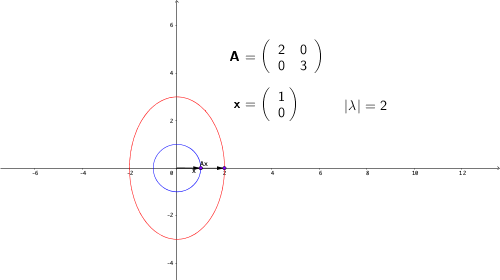 Figure 12.6: Eigenvalue of a diagonal matrix
 Figure 12.7: Eigenvalues of non-diagonal matrices
Suppose that we find \(n\) distinct eigenvectors \(\{\mathbf{v}_{i}\}_{i=1,\dots,n}\) with \(n\) distinct real-valued eigenvalues, then the transformation \(\mathbf{A}\) is decomposable into \(n\) one-dimensional transformations acting along the \(\mathbf{v}_{1}, \dots, \mathbf{v}_{n}\) axes: \[\mathbf{A}\mathbf{v}_{1}=\lambda_{1}\mathbf{v}_{1},\;\dots,\;\mathbf{A}\mathbf{v}_{n}=\lambda_{n}\mathbf{v}_{n}.\] This result implies that given an indecomposable non-diagonal matrix \(\mathbf{A}\), it is possible to find new axes, along which the matrix behaves as diagonalizable one. The new axes, namely the eigenvectors \(\{\mathbf{v}_{1},\dots,\mathbf{v}_{n}\}\) constructs a new coordinate system.228 Formally speaking, \(\mathbf{v}_{1}, \dots, \mathbf{v}_{n}\) will construct a basis in a finite dimensional vector space \(\mathcal{V}\). Any point in \(\mathcal{V}\) can be uniquely represented by a linear combination of \(\mathbf{v}_{1}, \dots, \mathbf{v}_{n}\). The coefficients of the linear combination are referred to as coordinates. And the basis is said to construct a coordinate system. The transformation \(\mathbf{A}\) can be fully interpreted under the new coordinate system.
The standard coordinate system is constructed by the standard unit vectors, i.e. \(\{\mathbf{e}_{1},\mathbf{e}_{2}\}\) in \(\mathbb{R}^{2}\), where \(\mathbf{e}_{1}=[1,0]^{\top}\) and \(\mathbf{e}_{2}=[0,1]^{\top}\). In the standard coordinate system, to get to any point of \(\mathbb{R}^{2}\) in this, one can choose to go a certain distance along \(\mathbf{e}_{1}\) (horizontally) and then a certain distance along \(\mathbf{e}_{2}\) (vertically). Under the coordinate system of the eigenvectors \(\{\mathbf{v}_{1},\mathbf{v}_{2}\}\), one can get to any point in \(\mathbb{R}^{2}\) by moving along the \(\mathbf{v}_{1}\) and \(\mathbf{v}_{1}\)-direction.
Consider the following example of the matrix \(\mathbf{A}\): \[\mathbf{A}=\left[\begin{array}{cc} 1 & 2\\ 4 & 3 \end{array}\right].\] The eigenvalues of this matrix is given by \[ \begin{align*} \mbox{det}(\lambda\mathbf{I}-\mathbf{A})=&\mbox{det}\left[\begin{array}{cc} \lambda-1 & -2\\ -4 & \lambda-3 \end{array}\right]\\=(\lambda-1)(\lambda-3)-8=&\lambda^{2}-4\lambda-5=(\lambda-5)(\lambda+1) \end{align*} \] with the solutions \(\lambda_{1}=5\) and \(\lambda_{2}=-1\). Then one can solve the two fixed point problems \((\mathbf{A}/5)\mathbf{v}_{1}=\mathbf{v}_{1}\) and \((\mathbf{A}/-1)\mathbf{v}_{2}=\mathbf{v}_{2}\) to find out the corresponding eigenvectors \(\mathbf{v}_{1}=[1,2]^{\top}\) and \(\mathbf{v}_{2}=[1,-1]^{\top}\).229 One can check that \[ \begin{align*} \left[\begin{array}{cc} 1 & 2\\ 4 & 3 \end{array}\right]\left[\begin{array}{c} 1\\ 2 \end{array}\right]&=5\left[\begin{array}{c} 1\\ 2 \end{array}\right],\\ \;\left[\begin{array}{cc} 1 & 2\\ 4 & 3 \end{array}\right]\left[\begin{array}{c} 1\\ -1 \end{array}\right]&=-1\left[\begin{array}{c} 1\\ -1 \end{array}\right]. \end{align*} \] The eigenvectors give a new coordinate system \(\{\mathbf{v}_{1},\mathbf{v}_{2}\}\) where we can navigate any point in \(\mathbb{R}^{2}\). For example, the point \(\mathbf{x}=[3,0]^{\top}\) under the \(\{\mathbf{v}_{1},\mathbf{v}_{2}\}\) is moved by one unit \(\mathbf{v}_{1}\)-direction and two units \(\mathbf{v}_{2}\)-direction from the origin, namely \[1\times\left[\begin{array}{c} 1\\ 2 \end{array}\right]+2\times\left[\begin{array}{c} 1\\ -1 \end{array}\right]=\left[\begin{array}{c} 3\\ 0 \end{array}\right].\] If the point is at \(\mathbf{A}\mathbf{x}=[3,12]^{\top}\), under the \(\{\mathbf{v}_{1},\mathbf{v}_{2}\}\)-coordinate it can be represented by is \([\mathbf{v}_{1},\mathbf{v}_{2}]\cdot[5,-2]^{\top}=5\mathbf{v}_{1}+2\mathbf{v}_{2}\) or written as the new coordinates \([5,-2]_{\{\mathbf{v}_{1},\mathbf{v}_{2}\}}\), namely, five units \(\mathbf{v}_{1}\) and negative two units \(\mathbf{v}_{2}\).
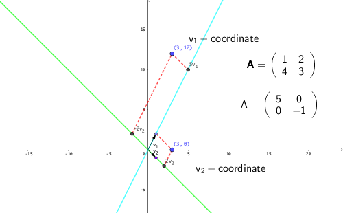 Figure 12.8: New coordinates
When the eigenvalues are complex numbers, the diagonalization still works, however it becomes difficult to represent in a 2D graph, as the transformation relating to the imaginary numbers is about the rotation, which cannot be decomposed in 1D.230 As shown in section 12.1, the rotation transformation has complex eigenvalues. Two real eigenvalues mean that the function could be decomposed into two 1D expansions or contractions, or into one saddle point (one expands and one contracts), but two complex eigenvalues make the transformation in a 4D space (two real and two imaginary axes). See figure 12.12 Because the complex eigenvalues of a transformation imply the existence of the rotation in this transformation, and because the eigenvectors are unchanged with the direction of the transformation, we can deduce that the associated eigenvectors will also need to be complex. That is to say, when a transformation involves rotations, then its eigenvalues and eigenvectors ought to be complex. For the \(2\times2\) matrix, diagonalization implies either two distinct real eigenvalues or a pair of complex conjugate eigenvalues. We can generalize the previous arguments to any square matrix.
If a matrix \(\mathbf{A}\) satisfied \(\mathbf{T}^{-1}\mathbf{A}\mathbf{T}=\mathbf{B}\) or \(\mathbf{A}=\mathbf{T}\mathbf{B}\mathbf{T}^{-1}\), then \(\mathbf{A}\) is said to be similar to matrix \(\mathbf{B}\). A matrix is diagonalizable if it is similar to a diagonal matrix.
- Diagonalization and similarity : For an \(n\times n\) matrix \(\mathbf{A}\), if \(\mathbf{A}\) has \(n\)-distinct eigenvectors such that \(\mathbf{A}\mathbf{v}_{1}=\lambda_{1}\mathbf{v}_{1}, \dots, \mathbf{A}\mathbf{v}_{n}=\lambda_{n}\mathbf{v}_{n}\), and \(\lambda_i \neq \lambda_j\) for any \(1\leq i,j\leq n\), then \(\mathbf{v}_{1},\dots,\dots\mathbf{v}_{n}\) are linearly independent and \(\mathbf{V}\) is invertible where \(\mathbf{V}=[\mathbf{v}_{1},\dots,\dots\mathbf{v}_{n}]\). Let \(\Lambda=\mbox{diag}\{\lambda_{1},\dots,\lambda_{n}\}\), the relation \(\mathbf{A}\mathbf{V}=\mathbf{V}\Lambda\) of eigenvectors and eigenvalues implies \[ \mathbf{V}^{-1}\mathbf{A}\mathbf{V}=\Lambda,\] which says that \(\mathbf{A}\) is similar to the diagonal matrix \(\Lambda\), namely \(\mathbf{A}\) is diagonalizable.
Any two similar matrices have the same eigenvalues and the same characteristic polynomial.231 In chapter 2.2, the cryptosystem is based on some kind of conjugate operation (to construct two similar system). The idea of this operation exactly follows the fact that encrypted system and the decrypted system share the same eigenvalues (the crypto information). Thus, if \(\mathbf{A}\) is diagonalizable, and \(\mathbf{A}\) is similar to \(\mathbf{B}\), one can infer that \(\mathbf{B}\) is also diagonalizable.
Proof
To see the use of diagonalization in dynamical systems, let’s recall that a matrix-vector multiplication can represent a dynamics of multiple inputs (see chapter 10.4). In the discrete linear dynamical system, with an initial vector \(\mathbf{x}_{0}\), the linear transformation \(\mathbf{A}\mathbf{x}_{1}=\mathbf{x}_{0}\) evokes the system. The iteration \(\mathbf{A}\mathbf{x}_{t}=\mathbf{x}_{t-1}\) can simulate the full set of dynamics of this system.
The computation of \(\mathbf{x}_{t}\) based on the initial vector \(\mathbf{x}_{0}\) requires \(t\) times iterations, namely \[\mathbf{x}_{t}=\mathbf{A}\mathbf{x}_{t-1}=\mathbf{A}(\mathbf{A}\mathbf{x}_{t-2})=\cdots=\mathbf{A}^{t}\mathbf{x}_{0}.\] To compute the power of matrices is not as simple as to compute the power of scalars.232 The issue is more serious if the power of matrices is used for linearization where a small perturbation may propogate unexpected chaotic consequences which makes the whole computational scheme fail. We will come to the topic of chaos in CH[?].. However, to compute the power of diagonal matrices is simple. For example: \[ \begin{align*} \Lambda^{k}&= \left[\begin{array}{ccc} \lambda_{1} & 0 & 0\\ & \ddots & 0\\ 0 & 0 & \lambda_{n} \end{array}\right]\times\left[\begin{array}{ccc} \lambda_{1} & 0 & 0\\ & \ddots & 0\\ 0 & 0 & \lambda_{n} \end{array}\right]\cdots\times\left[\begin{array}{ccc} \lambda_{1} & 0 & 0\\ & \ddots & 0\\ 0 & 0 & \lambda_{n} \end{array}\right]\\ &= \left[\begin{array}{ccc} \lambda_{1}^{k} & 0 & 0\\ & \ddots & 0\\ 0 & 0 & \lambda_{n}^{k} \end{array}\right]=\mbox{diag}\{\lambda_{1}^{k},\dots,\lambda_{n}^{k}\}. \end{align*} \] Thus, if the matrix is diagonalizable with the eigenvector matrix \(\mathbf{V}\) and the eigenvalue matrix \(\Lambda\), we may expect to have \[\mathbf{A}^n = (\mathbf{V}^{-1}\Lambda\mathbf{V})^n=(\mathbf{V}^{-1}\Lambda\mathbf{V}\mathbf{V}^{-1}\Lambda\mathbf{V}\cdots\mathbf{V}^{-1}\Lambda\mathbf{V})=\mathbf{V}^{-1}\Lambda^n\mathbf{V}.\] In this case, the advantage is clear: we need to calculate and apply the eigenvector matrix \(\mathbf{V}\) and \(\mathbf{V}^{-1}\) only once, and the rest of the iteration process is simply applying the \(n\)-th power of the diagonal matrix \(\Lambda\).
Apart from the computational advantage, the diagonalization also assists us to disentangle some complex dynamical patterns of the coupled systems. In chapter 4.3 and 8.2, we have seen what a univariate (1D) time series is. The four possible dynmaical patterns of \(x_t = \lambda x_{t-1}\) are summarized in figure 12.9.233 The figure is designed for \(\mathbf{x}_{1,t}=0.8\mathbf{x}_{1,t-1}\), \(\mathbf{x}_{2,t}=1.02\mathbf{x}_{2,t-1}\), \(\mathbf{x}_{3,t}=-0.8\mathbf{x}_{3,t-1}\) and \(\mathbf{x}_{4,t}=-1.02\mathbf{x}_{4,t-1}\). We can see that the series converges if \(|\lambda|<1\) and diverges if \(|\lambda|>1\). For negative \(\lambda\), the trends oscillate; for positive \(\lambda\), the trends are monotonic.
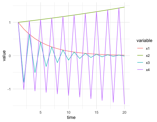 Figure 12.9: Dynamical patterns
Code
For a \(2\times2\) diagonal matrix \(\mathbf{A}\), its linear dynamical system \(\mathbf{x}_{t}=\mathbf{A}\mathbf{x}_{t-1}\) only consists of two seperated univariate time series. This kind of system is called the uncoupled system where the growth of one series only depends on its own historical states. On the other hand, if the off-diagonal entries of \(\mathbf{A}\) are non-zero, then the dynamical system is a coupled system. The diagonalization allows us to analyze a coupled system in its uncoupling form.
Consider the following system \[ \left[\begin{array}{c} x_{1,t}\\ x_{2,t} \end{array}\right]=\mathbf{A}\mathbf{x}_{t-1}=\left[\begin{array}{cc} 0.65 & 0.5\\ 0.25 & 0.9 \end{array}\right]\left[\begin{array}{c} x_{1,t-1}\\ x_{2,t-1} \end{array}\right] \] The eigenvalues of this system are \(\lambda_{1}=1.15\), and \(\lambda_{2}=0.4\). The eigenvectors can be chosen to be \(\mathbf{v}_{1}=[1,1]^{\top}\) and \(\mathbf{v}_{2}=[-2,1]^{\top}\). Notice that the eigenvalues are real numbers and \(|\lambda_{1}|>1\) and \(\lambda_{2}|<1\). So for the uncoupled system \((\mathbf{V}\mathbf{x}_{t})=\Lambda(\mathbf{V}\mathbf{x}_{t-1})\), we expect the behavior of the system must expand along the \(\mathbf{v}_{1}\)-coordinate and contract along the \(\mathbf{v}_{2}\)-coordinate. Figure 12.10 shows that the initial vector \(\mathbf{x}_{0}= [10,50]^{\top}\) grows along the \(\mathbf{v}_{1}\)-coordinate in five periods.
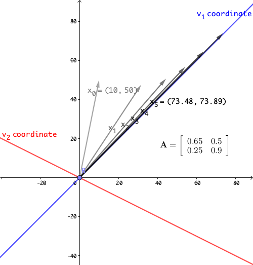 Figure 12.10: Linear dynamical system 1
 Figure 12.11: Linear dynamical system 2
Consider another system \[ \left[\begin{array}{c} x_{1,t}\\ x_{2,t} \end{array}\right]=\mathbf{A}\mathbf{x}_{t-1}=\left[\begin{array}{cc} 0.1 & 1.4\\ 0.4 & 0.2 \end{array}\right]\left[\begin{array}{c} x_{1,t-1}\\ x_{2,t-1} \end{array}\right] \]
The eigenvalues of this system are \(\lambda_{1}=0.9\), and \(\lambda_{2}=-0.6\). The eigenvectors can be chosen to be \(\mathbf{v}_{1}=[1,1]^{\top}\) and \(\mathbf{v}_{2}=[-2,1]^{\top}\). Figure 12.11 shows that the trend shrinks along \(\mathbf{v}_{1}\) but collapse in an oscillating manner along the \(\mathbf{v}_{2}\)-axis. The presence of oscillation is due to the negative eigenvalue which means that the matrix will flip the state point back and forth on either side of the \(\mathbf{v}_{1}\)-axis. The oscillation is diminishing because the largest absolute eigenvalue is less than one (otherwise, the oscillation will departure).
Derivations
 Figure 12.12: Linear dynamical system 3
The final case is that \(\lambda_1\) and \(\lambda_2\) are a pair of complex conjugate eigenvalues, and then the action of the matrix was a rotation. Recall the rotation matrix in section 12.1. If we set the angle of the rotation to \(120^{\circ}\), the matrix gives the following system: \[ \left[\begin{array}{c} x_{1,t}\\ x_{2,t} \end{array}\right]=\mathbf{A}\mathbf{x}_{t-1}=\left[\begin{array}{cc} 0 & 1\\ -1 & -1 \end{array}\right]\left[\begin{array}{c} x_{1,t-1}\\ x_{2,t-1} \end{array}\right] \] with the eigenvalues \(\lambda = \cos120^{\circ} \pm \mbox{i}\sin120^{\circ}= -\frac{1}{2} \pm \mbox{i}\frac{\sqrt{3}}{2}\), and the corresponding eigenvectors \(\mathbf{v}=[1,\pm\mbox{i}]^\top\). In figure 12.12 we apply this transformation with an initial vector \([5,0]^{\top}\), the complex eigenvalues induces rotations to the system. Because the absolute value of \(\lambda\) is \(\sqrt{\sin^2120^{\circ}+\cos^{2}120^{\circ}}=1\), these rotations neither expand nor shrink the sizes of the system. In other words, \(\mbox{e}^{\mbox{i}120^{\circ}} \mathbf{v}\) is to rotate \(120^{\circ}\) degrees along the “imaginary” coordinates \(\mathbf{v}=[1,\pm\mbox{i}]^\top\) that cannot be visualized in a 2D graph.
With above three examples, we can almost infer the following properties about the linear dynamical systems \(\mathbf{x}_t= \mathbf{A} \mathbf{x}_{t-1}\). Given the eigenvalue-eigenvector decomposition \(\mathbf{A}\mathbf{v}=\lambda\mathbf{v}\) If an eigenvalue of \(\mathbf{A}\) has absolute value less than \(1\), the matrix shrinks vectors lying along that eigenvector \(\mathbf{v}\). If the eigenvalue has absolute value greater than \(1\), the matrix expands vectors lying along that eigenvector. If the eigenvalue is negative, the action of the matrix is to flip back and forth between negative and positive values along that eigenvector. If the eigenvalue is a complex numbers \(z\), the polar form \(z=r\mbox{e}^{\mbox{i}\theta}\) seperates the rotation \(\mbox{e}^{\mbox{i}\theta}\) from the absolute size \(r\). In this case, the absolute value of \(r\) will indicate whether the matrix will shrink or will expand vectors, and \(\mbox{e}^{\mbox{i}\theta}\) will rotate vectors around the axis of the complex-valued eigenvector.
Let’s define the principal eigenvector as the eigenvector whose eigenvalue has the largest absolute value. In the linear dynamical system, the state will evolve until its motion lies along the principal eigenvector. The largest eigenvalue, as the principal eigenvalue will determine the long-term behavior of the iteration, i.e. expansion, contraction, rotation, etc.
Recall that for a single differential equation \(\mbox{d}x(t)/\mbox{d}t=\lambda x(t)\) with an initial value \(x(0)\), the solution is \(x(t)=x(0)\mbox{e}^{\lambda t}\). Similarly, for a linear system of differential equations, the diagonal matrix uncouples the system. Let \[\left[\begin{array}{c} \mbox{d}v_{1}(t)/\mbox{d}t\\ \mbox{d}v_{2}(t)/\mbox{d}t \end{array}\right]=\Lambda\mathbf{v}(t)=\left[\begin{array}{cc} \lambda_{1} & 0\\ 0 & \lambda_{2} \end{array}\right]\left[\begin{array}{c} v_{1}(t)\\ v_{2}(t) \end{array}\right].\] Suppose the initial vector is \([v_{1}(0),v_{2}(0)]^{\top}\), the above system can be treated as two seperated differential equations whose solution vector is \[\left[\begin{array}{c} v_{1}(t)\\ v_{2}(t) \end{array}\right]=\left[\begin{array}{c} v_{1}(0)\mbox{e}^{\lambda_{1}t}\\ v_{2}(0)\mbox{e}^{\lambda_{2}t} \end{array}\right],\] where \(\lambda_{1}\) and \(\lambda_{2}\) play the roles of growth rates for these differential equations.
Now we consider the third example of the linear dynamical system but under the continuous time setting. Let the matrix \(\mathbf{A}\) be the \(120^{\circ}\)-rotation matrix so that the system becomes: \[ \left[\begin{array}{c} \mbox{d}x_{1}(t)/\mbox{d}t\\ \mbox{d}x_{2}(t)/\mbox{d}t \end{array}\right]=\left[\begin{array}{c} x_{2}(t)\\ -x_{1}(t)-x_{2}(t) \end{array}\right]=\left[\begin{array}{cc} 0 & 1\\ -1 & -1 \end{array}\right]\left[\begin{array}{c} x_{1}(t)\\ x_{2}(t) \end{array}\right]. \] As we already knew the eigenvalues of this matrix are \(\lambda = -\frac{1}{2} \pm \mbox{i}\frac{\sqrt{3}}{2}\), we can infer the trends of this dynamical system. Notice that unlike in the discrete time setting, the solution vector contains \(\mbox{e}^{\lambda t}\), the exponential function of complex eigenvalues \(\lambda\).234 This difference is due to the differential operator. In fact, we can extend the idea to general linear mappings or operators. Take the differential operator \(\frac{\mbox{d}}{\mbox{d}x}\) (the operation of taking the derivative of a function) as an example. As the operation is linear, one may also expect there exist some “eigenvector” (or formally eigenfunction) of the operator. Let \(v(x)=\mbox{e}^{\lambda x}\). We know that \[\frac{\mbox{d}}{\mbox{d}x}v(x)=\lambda v(x).\] In other words, the exponential function \(\mbox{e}^{\lambda x}\) is an eigenvector to the derivative-operator with eigenvalue \(\lambda\). We will come back to this point in Ch[?]. . The exponential function can be decomposed into two parts \[\mbox{e}^{\lambda t}=\mbox{e}^{-\frac{t}{2}} \mbox{e}^{\pm \mbox{i}\frac{\sqrt{3}}{2} t},\] a real exponential function and a pair of exponential functions with conjugate imaginary numbers. According to the previous discussion on convergences of differential equations in chapter 8.1, the real negative (positive) growth rate indicates the convergent (divergent) trend. Because the real parts of the eigenvalues are less than zero, we expect the system to converge. Because of the imaginary term \(\mbox{e}^{\pm \mbox{i}\frac{\sqrt{3}}{2} t}\), we also expect some rotations of \(x_1(t)\) and \(x_2(t)\) occuring in the process of convergence. In figure 12.13, we can find that both solutions converge to zero. The convergence accompanies with some oscillationary movements across time \(t\). The oscillation is caused by the rotation. Because the rotation (of a 2D circle) means the loss or the gain in one direction is partially compensated by the gain or the loss from the other. This rotation together with the convergent treand appears as a stable spiral in figure 12.14. Figure 12.14 provides a coordinate plane with axes being the values of two state variables \(x_1(t)\) and \(x_2(t)\). This kind of plots is called the phase plot.
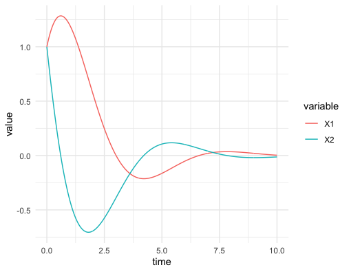 Figure 12.13: Solutions
 Figure 12.14: Phase plot of the solutions
Code of solving the simple ODE system
12.3 * Miscellaneous: Alchemy and Values
Alchemy is about an idea of a common metallic matter subject to interchangeable sets of qualities. The common metallic matter in the west was called Philosophers’ stone, and in the east was called Golden elixir. They both reveal an ideal capability of transforming substances. While Philosophers’ stone is supposed to transform the substances into better ones, the Golden exlixir is supposed to transform the substances into immortal ones. In history, legions of alchemists sought for these stones to transform coloring metals, stones, and cloth into precious (or apparently precious) objects.
Transformation, as an alchemical theme here, obeys a cosmic view of the world that all substances are composed of the same fundamental one. If a single material that serves as the fundamental for all substances, one may expect to turn one thing into another because at the deepest level they are really the same thing. In Greek philosophy, this idea is the ladder of nature: everything in existence, from inanimate matter to the transcendent one, is linked in a hierarchical chain. In Chinese philosophy, this idea is called the correlative cosmology (天人合一): all entities and phenomena ultimately originate from the Dao (道) in a hierarchical manner.235 This idea later was developped into a doctrine called interactions between heaven and mankind (天人感应) by the confucian politician Dong Zhongshu. The doctrine approached within the ace of the Christian faith where the omniscience of God implied that a uniform, harmonious, interfunctioning world, namely a highly ordered and self-consistent whole. It not only served as a basis for deciding the legitimacy of Chinese monarch but also provided governing guidances on a reigning monarch. These principles undergirded the idea of alchemical transmutation, and encourged alchmists to explore the theoretical possibility of transforming unessential substances into more valuable ones.
From my current point of view, the literature about alchemy consists of a forbidding tangle of intentional secrecy, bizarre ideas, and strange images plunging the readers into a maze of conflicting claims and contradictory assertions. Thus, my motivation is not to provide any serious knowledge about the secrets, the processes or the privileges of alchemy, as I think the comprehensive root of the subject has been merged into modern chemistry. Instead, I will treat the alchemy as a kind of exploration of the nature of matter under the themes of purification and improvement. And by giving a brief retrospective description of this exploration, I will provide a coarse outline of defining the value (of transformations) from an alchemical perspective.
Alchemy, like other sceintific pursuits, has a skeleton of theory that provides intellectual fundamentals, that instructs the practical works, and illuminates the perspicuous pathways of future developments. Ancient Greek philosophers (Empedocles and later Aristotle) attributed the origin of natural substances and their transformations to four “roots” of things which are fire, air, earth, and water. Similarly, ancient Chinese philosophers attributed the essence, namely the set of properties constructing substances, to five elements which are earth, metal, water, wood, and fire. Both schools of thoughts endeavored to explain matter’s hidden nature and to account for its unending transformations into new forms. Most of the following ideas point to the belief that some sort of an invariant hidden beneath the constantly changing appearances of things. The invariant of Thales was water, of Aristotle was the first matter, of Empedocles were four elements, of Daoists and Confucianists were five elements.
Just like any current empirical research activities, alchemists relied on those theoretical principles to guide the practical work. The practice of transformative process could involve special psychic states and incorporeal agents. The history of alchemy were simultaneously chemical, spiritual, and psychological, but that the main purpose of those pratical works looked like to unite the several constituents of consciousness and to develop a trascending state of mankind. At this point, we can see a clear bifurcation of two schools.
Judaic-Christian alchemy: The Philosophers’ stone as a perfect metal represents the state of quintessence for transforming corrodible base metals into incorruptible gold.236 The metals were divided into different categories. By the standards of the intrinsic beauty and the ability to resist corrosion, noble metals (such as gold and silver) are different from the base metals (such as copper, iron, tin, lead, and mercury).
Chinese alchemy: The Golden elixir as a immortal pellet represents the state of constancy and immutability beyond the change and transiency.237 In Chinese history, Sulphur and nitre were both used for medicinal purposes to extend the life of a person, and for military purposes to extend the life of the culture.
Even though the ultimal goals looked different, if we interpret the chemical processes declared by the alchemists as metaphorical or analogical manifestations of the need for enhancing knowledge to achieve salvation, of the need for distilling human’s inner being to archieve divinity, we may consider what all these alchemists sought were the same, a purely self-transformative, meditative, psychic process.238 Jung (2008) asserted that the real object of alchemy was the transformation of the psyche, and considered Alchemy’s “true root” was to be found not so much in philosophical ideas and outlooks but rather in “experiences of projection of the individual researcher.” Jung (2008) say, “a peculiar attitude of the mind—the concentration of attention on a single thing. The result of this state of concentration is that the mind is absorbed to the exclusion of other things, and to such a degree insensible that the way is opened for automatic actions; and these actions, becoming more complicated, as in the preceding case, may assume a psychic character and constitute intelligences of a parasitic kind, existing side by side with the normal personality, which is not aware of them.” Since the psyche could project its contents onto any sort of matter, the actual substances employed by the alchemist were not crucial. Jung believe that Alchemy’s allegorical language were expressions of a collective unconscious.
Transformation, in a alchemical metaphor, could be about the changes of the non-volatile body and the volatile spirit. The body seems to be the same for all substances; so the identity is dependent on its spirit.
The Judaism-Christian alchemy focused on a transformation from a state of nature to a state of grace by releasing the imprisoned material body. Themes such as purification and distillation readily lend themselves as moral or spiritual symbols. Knowledge, in this case, was necessary to overcome one’s ignorance, to liberate oneself from the material world and the evil forces.
The Chinese alchemy focused on a transformation from a fleeting state to an eternal state by collecting the seperated spirits. Metaphorical sublimation and volatilization seperated the spirits from the various bodies. Joining the separated temporary spirits formed a unified long-lived consciousness, and established the desired collective knowledge.
All these alchemical reactions nowadays were thought to be chemical related reactions. It may be interesting to know that an overall chemical reaction consists of a finite number of individual reaction steps that can be represented by a matrix equation \(\mathbf{A}\mathbf{x}=0\), where \(\mathbf{A}=[a_{ij}]_{n\times m}\), \(m\) stands for the number of different chemical species, \(n\) stands for the number of different reactions, and \(\mathbf{x}=[x_{j}]_{m\times1}\) represents the concentrations of \(m\) chemical species. The matrix \(\mathbf{A}\) is called the stoichiometric matrix that shows certain linear combinations of concentrations.239 An stoichiometric equation comes with a reaction arrow, left of which gives the substances with negative stoichiometric coefficients (reactants), and right of which gives the substances with positive stoichiometric coefficients (products). For example a chemical reaction \(x_{1}+3x_{2}\rightarrow2x_{3}\) is represented by \(-x_{1}-3x_{2}+2x_{3}=0\). The theory of this model is known as the chemical reaction network theory. Then the same stoichiometric matrix can describe the dynamical changes of a system of elementary reactions in a system of differential equations, such as \(\mbox{d}\mathbf{x}(t)/\mbox{d}t=\mathbf{A}f(\mathbf{x}(t))\), where \(f(\cdot)\) is a function about the rate of reactions.240 Usually, the function \(f(\cdot)\) adheres to a power law of the kinetic energy, which means that \(f(x_{i})\) is obtained by multiplying the concentrations raised to a suitable power (a monomial), i.e. \(f(x_{i})=c_{i}\prod_{k=1}^{m}x_{k}^{\beta_{j,k}}\). Then one can have a multivariate polynomial where the \(i\)-entry of \(\mathbf{A}f(\mathbf{x}(t))\) is given by \(\sum_{j=1}^{n}a_{ij}c_{i}\prod_{k=1}^{m}x_{k}^{\beta_{j,k}}\). The equations \(\mathbf{A}f(\mathbf{x}(t))\) typically preserve the autonomous property of differential equations. A reaction step with this power law can be written as the following chemical equation: \(\sum_{j=1}^{m}\beta_{ij}x_{j}\rightarrow\sum_{j=1}^{m}(\beta_{ij}+a_{ij})x_{j}\).
Unfinished!
Will come back later!
12.4 Example: Matrix Norm, Changes of Basis, Autoregressive Model, Trade Flows
Matrix norm
The concept of a vector norm gives us a way of thinking about the “size” of a vector. We could easily extend this to matrices, just by thinking of a matrix as a vector that had been chopped into segments of equal length and then re-stacked as a matrix. Thus, every vector norm on the space \(\mathbb{R}^{m\times n}\) of vectors of length \(m\times n\) gives rise to a vector norm on the space of \(m\times n\) matrices. Since the abosulte value of the eigenvalue is a real number, a nautral idea is to let the eigenvalue serve the role as a matrix norm. Unfortunately, the experience has shown that this is not the best way to look for norms of matrices because of the operation of matrix multiplication. In a matrix-vecotr multiplication, a matrix linearly transforming a vector into another one can rescale the norms of these vectors. By taking the vector norms of the eigenvalue-eigenvector decomposition \(\|\mathbf{A} \mathbf{v} \| = \|\lambda \mathbf{v}\|\), we can see that given \(\mathbf{A}\), the absolute value \(|\lambda| = \| \mathbf{A} \mathbf{v} \|/ \| \mathbf{v} \|\) varies with the vector \(\mathbf{v}\) (see figure 12.7).
The reason is that any linear combination of eigenvectors \(\mathbf{v}\) can provide a corresponding eigenvalue \(\lambda\). Then, there could be infinite absolute \(\lambda\)s of a matix transformation, while the norm is a function whose output is set to a single real-valued number. Fortunately, for any set of real numbers, by the axiom of completeness of real numbers, such a set is bounded above and has a supremum. Thus, we need to take the supremum of all possible real-valued \(|\lambda|\)s to attain a unique output. Here is a usual definition of the (strong) matrix norm241 Similarly, as the operator is the counterpart of a matix in the finite dimension, the norm of the operator \(\mathbf{T}_{\mathbf{A}}\) can be induced by the matrix norm such that \[\|\mathbf{T}_{\mathbf{A}}\|=\sup_{\mathbf{x}\neq0}\frac{\|\mathbf{T}_{\mathbf{A}}(\mathbf{x})\|}{\|\mathbf{x}\|}.\]: \[\|\mathbf{A}\|=\sup_{\mathbf{x}\neq0}\frac{\|\mathbf{A}\mathbf{x}\|}{\|\mathbf{x}\|}.\]
Changes of basis
Recall that the diagonalization of an \(n \times n\) square matrix \(\mathbf{A}\) means that \(\mathbf{A}\) is similar to the diagonal eigenvalue matrix \(\Lambda=\mbox{diag}\{\lambda_{1},\dots,\lambda_{n}\}\), such that \(\mathbf{V}^{-1}\mathbf{A}\mathbf{V}=\Lambda\) or \(\mathbf{A}=\mathbf{V}\Lambda\mathbf{V}^{-1}.\) If another matrix \(\mathbf{B}\) is similar \(\mathbf{A}\), say \(\mathbf{X}^{-1}\mathbf{B}\mathbf{X}=\mathbf{A}\) or \(\mathbf{B}=\mathbf{X}\mathbf{A}\mathbf{X}^{-1}\), then it is easy to see that \(\mathbf{A}\) and \(\mathbf{B}\) have the same eigenvalues and the same characteristic polynomial.242 By properties of determinants and the trick \(\mathbf{X}^{-1}\mathbf{I}\mathbf{X}=\mathbf{I}\), we have \[ \begin{align*} \mbox{det}(\lambda\mathbf{I}-\mathbf{A})&=\mbox{det}(\lambda\mathbf{X}^{-1}\mathbf{I}\mathbf{X}-\mathbf{X}^{-1}\mathbf{B}\mathbf{X})\\&=\mbox{det}(\mathbf{X}^{-1}(\lambda\mathbf{I}-\mathbf{B})\mathbf{X})\\ &=\mbox{det}(\mathbf{X}^{-1})\mbox{det}(\lambda\mathbf{I}-\mathbf{B})\mbox{det}(\mathbf{X})\\&=\mbox{det}(\lambda\mathbf{I}-\mathbf{B}). \end{align*} \] So the characteristic polynomials of \(\mathbf{A}\) and \(\mathbf{B}\) are the same. In this case, we have \[\mathbf{B}=\mathbf{X}\mathbf{A}\mathbf{X}^{-1}=(\mathbf{X}\mathbf{V})\Lambda(\mathbf{V}^{-1}\mathbf{X}^{-1})=(\mathbf{X}\mathbf{V})\Lambda(\mathbf{X}\mathbf{V})^{-1},\] where the matrix \(\mathbf{X}\) is viewed as a change of basis matrix from the basis of \(\mathbf{A}\), namely \(\mathbf{V}\), to another basis of \(\mathbf{B}\), namely \(\mathbf{X}\mathbf{V}\). Any linear operation of changing basis follows this idea of preserving the invariant eigenvalues.
To generalize this idea, we can change the basis of two polynomial matices. First, we show that when a matrix is mapped by a polynomial function, the eigenvalue matrix is simultaneously mapped by the same function. Let \(f(z)=c_{0}+c_{1}z+\cdots+c_{n}z^{n}\) be a polynomial function, it is easy to see that when the input is a diagonal matrix, the function \(f(\Lambda)\) is another diagonal matrix with entries as polynomials such that \(f(\Lambda)=\mbox{diag}\{f(\lambda_{1}),\dots,f(\lambda_{n})\}\).243 Functions like \(\sin(\cdot)\), \(\cos(\cdot)\) and \(\mbox{e}^{(\cdot)}\), which do not appear as polynomials but can be defined in terms of power series (the infinite version of a polynomial function) can also have such property.
To see this argument, we know that \[f(\Lambda)=c_{0}\mathbf{I}+c_{1}\Lambda+\cdots+c_{n}\Lambda^{n}.\] Each monomial \(\Lambda^{k}\) has the following expression \[\Lambda^{k} = \left[\begin{array}{ccc} \lambda_{1}^{k} & 0 & 0\\ & \ddots & 0\\ 0 & 0 & \lambda_{n}^{k} \end{array}\right]=\mbox{diag}\{\lambda_{1}^{k},\dots,\lambda_{n}^{k}\}.\] So adding up all the monomials gives \[ \begin{align*} f(\Lambda) &= c_{0}\left[\begin{array}{ccc} 1 & 0 & 0\\ & \ddots & 0\\ 0 & 0 & 1 \end{array}\right]+c_{1}\left[\begin{array}{ccc} \lambda_{1} & 0 & 0\\ & \ddots & 0\\ 0 & 0 & \lambda_{n} \end{array}\right]+\cdots+c_{n}\left[\begin{array}{ccc} \lambda_{1}^{n} & 0 & 0\\ & \ddots & 0\\ 0 & 0 & \lambda_{n}^{n} \end{array}\right] \\ &= \left[\begin{array}{ccc} c_{0}+c_{1}\lambda_{1}+\cdots c_{n}\lambda_{1}^{n} & 0 & 0\\ & \ddots & 0\\ 0 & 0 & c_{0}+c_{1}\lambda_{n}+\cdots+c_{n}\lambda_{n}^{n} \end{array}\right]\\ &=\left[\begin{array}{ccc} f(\lambda_{1}) & 0 & 0\\ & \ddots & 0\\ 0 & 0 & f(\lambda_{n}) \end{array}\right]. \end{align*} \] When \(\mathbf{A}\) is diagonalizable as \(\mathbf{V}^{-1}\mathbf{A}\mathbf{V}=\Lambda\), for any monomial \(\Lambda^{k}\) in \(f(\Lambda)\), we have \[\Lambda^{k}=(\mathbf{V}^{-1}\mathbf{A}\mathbf{V})(\mathbf{V}^{-1}\mathbf{A}\mathbf{V})\cdots(\mathbf{V}^{-1}\mathbf{A}\mathbf{V})=\mathbf{V}^{-1}\mathbf{A}^{k}\mathbf{V}.\] The eigenvalue-eigenvector decomposition becomes \(f(\mathbf{A})\mathbf{V}=f(\Lambda)\mathbf{V}\) or \(\mathbf{V}^{-1}f(\mathbf{A})\mathbf{V}=f(\Lambda)\) because \[f(\Lambda)=c_{0}+c_{1}\Lambda+\cdots+c_{n}\Lambda^{n}=\mathbf{V}^{-1}(c_{0}+c_{1}\mathbf{A}+\cdots+\mathbf{A}^{n})\mathbf{V}=\mathbf{V}^{-1}f(\mathbf{A})\mathbf{V}.\] In other words, the diagonalization of the polynomial matrix \(f(\mathbf{A})\) is \[f(\Lambda)=\mathbf{V}^{-1}f(\mathbf{A})\mathbf{V}.\] Therefore, if \(\mathbf{B}\) is similar to \(\mathbf{A}\) in terms of \(\mathbf{X}^{-1}\mathbf{B}\mathbf{X}=\mathbf{A}\), we can induce that for any polynomial function \(f(\cdot)\), \(f(\mathbf{B})\) is similar to \(f(\mathbf{A})\) in terms of \(\mathbf{X}^{-1}f(\mathbf{B})\mathbf{X}=f(\mathbf{A})\). The change of basis follows the same structure: \[f(\mathbf{B})=\mathbf{X}f(\mathbf{A})\mathbf{X}^{-1}=(\mathbf{X}\mathbf{V})f(\Lambda)(\mathbf{X}\mathbf{V})^{-1}.\]
In addition, the basis \(\mathbf{X}\) and \(\mathbf{V}\) can also be interchanged with each other. Consider an example in \(\mathbb{R}^{2}\). For two coordinate systems, say \(\{\mathbf{x}_{1},\mathbf{x}_{2}\}\) and \(\{\mathbf{v}_{1},\mathbf{v}_{2}\}\), there must exist a linear combination of \(\mathbf{v}_{1}\) and \(\mathbf{v}_{2}\) for representing \(\mathbf{x}_{1}\) under the \(\{\mathbf{v}_{1},\mathbf{v}_{2}\}\)-coordinate, so does for representing \(\mathbf{x}_{2}\): \[ \begin{align*} \mathbf{x}_{1} &= c_{11}\mathbf{v}_{1}+c_{21}\mathbf{v}_{2}\\ \mathbf{x}_{2} &= c_{12}\mathbf{v}_{1}+c_{22}\mathbf{v}_{2}. \end{align*} \] In other words,\[[\mathbf{x}_{1},\mathbf{x}_{2}]=[\mathbf{v}_{1},\mathbf{v}_{2}]\left[\begin{array}{cc} c_{11} & c_{12}\\ c_{21} & c_{22} \end{array}\right]=[\mathbf{v}_{1},\mathbf{v}_{2}]\mathbf{C},\] where the matrix \(\mathbf{C}\) is called the change of basis transformation.
Example of the change of basis transformation
Autoregressive model
In the linear regression example in chapter 10.2, we have seen the way of finding a linear relation between a data vector \(\mathbf{x}\) and \(\mathbf{y}\) by \(\mathbf{y} = \hat{\beta}\mathbf{x}\) where \(\hat{\beta}\) is the estimator given by the projection formula.
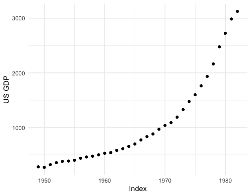 Figure 12.15: US GDP
Now let’s switch our attention to some real dynamical data (time series data), and we can find that this regressive idea still works. The idea of autoregression is about regressing a data vector on itself. Consider one time series \(\{x_{t}\}_{t=1,\dots,T}\) as a vector \(\mathbf{x}_{T}=[x_{1},\dots,x_{T}]^{\top}\). we can shift \(\mathbf{x}_{T}\) to \(\mathbf{x}_{T-1}=[0,x_{2},\dots,x_{T-1}]^{\top}\) by using a lagged operation matrix (a lower triangular elementary matrix) \(\mathbf{L}\) such that \[\mathbf{L}\mathbf{x}_{T}=\left[\begin{array}{ccccc} 0 & 0 & 0 & \cdots & 0\\ 1 & 0 & 0 & \cdots & 0\\ 0 & 1 & 0 & \cdots & \vdots\\ \vdots & & \ddots & \ddots & 0\\ 0 & 0 & \cdots & 1 & 0 \end{array}\right]\left[\begin{array}{c} x_{1}\\ x_{2}\\ \vdots\\ x_{T} \end{array}\right]=\left[\begin{array}{c} 0\\ x_{1}\\ \vdots\\ x_{T-1} \end{array}\right]=\mathbf{x}_{T-1}.\]
We call \(\mathbf{x}_{T-1}\) the lagged vector of \(\mathbf{x}_{T}\). Then a difference equation \(x_{t}=\phi x_{t-1}\) for \(t=1,\dots T\) can be expressed by a single relation between the data vector \(\mathbf{x}_{T}\) and its lagged vector \(\mathbf{x}_{T-1}\) such that \(\mathbf{x}_{T}=\phi\mathbf{x}_{T-1}=\phi\mathbf{L}\mathbf{x}_{T}\) or \[\mathbf{L}\mathbf{x}_{T}= \lambda \mathbf{x}_{T}\] where \(\lambda = \phi^{-1}\) plays as a similar role as the eigenvalue of the lagged operation matrix, and \(\mathbf{x}_{T}\) plays the role as the associated eigenvector.244 If we consider an infinite long time series \(\{x_{t}\}_{t\in\mathbb{N}^{+}}\), then we use an lagged operator \(\mathbf{T}_\mathbf{L}\) such that \(\mathbf{T}_\mathbf{L}\mathbf{x}_{t}=\mathbf{x}_{t-1}\). The statements and results are similar to those in the finite dimensional case.
For a real data vector, the entries may have been contaminated by some errors, so the projection formula can gives us the estimator \(\hat{\phi}\) of the autoregressive model \[\mathbf{x}_{T}=\phi\mathbf{x}_{T-1} + \mathbf{e}\] where \(\mathbf{e}\) is a vector of errors.
## [1] 1.04026In section 12.2, we have seen that to have a divergent (convergent) pattern, the absolute value of the coefficient needs to be greater than one (less than one), namely \(|\phi|>1\) or \(|\lambda| < 1\) (\(|\phi|<1\) or \(|\lambda| > 1\)).
Plot the estimated U.S. GDP
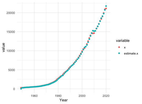 Figure 12.16: US GDP and the estimated values
The previous regression model uses one lagged vector, so it is often called an AR(1) (autoregressive model with one lagged variable). By multiplying the lagged operation matrix \(k\)-times, one can shift \(\mathbf{x}_{T}\) to \(\mathbf{x}_{T-k}=[0,\dots,x_{1},\dots,x_{T-k}]^{\top}\). So if one prefers to consider some relation depending on the longer historical information, one can regress on other lagged data vectors. For example, the relation \[x_{t}=\phi_{1}x_{t-1}+\phi_{2}x_{t-2}\] can induce an AR(2) model. However, it may be not so obvious to judge the dynamical pattern for this AR(2) model, as the eigenvalues of this model relate to the solution of a second order polynomial equation. To see this, we rewrite the relation of AR(2) as \[\mathbf{x}_{T}-\phi_{1}\mathbf{L}\mathbf{x}_{T}-\phi_{2}\mathbf{L}^{2}\mathbf{x}_{T}=f(\mathbf{L})\mathbf{x}_{T}=0\] where \(f(\mathbf{L})=1-\phi_{1}\mathbf{L}-\phi_{2}\mathbf{L}^{2}\). The eigen decomposition gives \(f(\mathbf{L})\mathbf{x}_{T}=f(\Lambda)\mathbf{x}_{T}\) where \(\Lambda=\mbox{diag}\{\lambda_1,\lambda_2\}\) is the eigenvalue matrix. The polynomial equation \(f(\mathbf{L})=0\) is equivalent to \(f(\Lambda)=0\) or say \(f(\Lambda)=\mbox{diag}\{f(\lambda_{1}), f(\lambda_{2})\}=0.\) Because the fundamental theorem of algebra asserts that the polynomial equation \(f(z)=0\) has two roots on the complex field, we can infer that \(\lambda_1\) and \(\lambda_2\) are these roots. That is to say, the second order polynomial equation can be factorized by two first order polynomial equations:245 The factor theorem of polynomials asserts that a polynomial of \(n\) order can be written as a product of two or more polynomials of degrees less than \(n\). Thus, if \(\lambda_{1}\), \(\lambda_{2}\) are two distinct roots of a second order polynomial \(f(z)\), then \(f(z)\) can be factorized as \(f(z)=c_{0}(z-\lambda_{1})(z-\lambda_{2})\). For the equation \(f(z)=0\), \(c_{0}\) does not matter, so we have \((z-\lambda_{1})(z-\lambda_{2})=0\). \[f(\mathbf{L})=(\mathbf{L} - \lambda_1)(\mathbf{L}-\lambda_2)=0,\] which implies that the AR(2) model \(f(\mathbf{L})\mathbf{x}_T = 0\) is equivalent to a system of two AR(1) models: \(\lambda_{1}\mathbf{x}_{T}=\mathbf{L}\mathbf{x}_{T}\) and \(\lambda_{2}\mathbf{x}_{T}=\mathbf{L}\mathbf{x}_{T}\). As we have seen in section 12.2, the property of such a dynamical system is controlled by the principal eigenvalue, namely \(\max\{|\lambda_{1}|,|\lambda_{2}|\}\). Similar to the AR(1) case, in order to have a converging (diverging) pattern, the principal eigenvalue of the lagged operation matrices needs to be greater than (less than) one, namely \(\max\{|\lambda_{1}|,|\lambda_{2}|\}>1\) (\(\max\{|\lambda_{1}|,|\lambda_{2}|\}<1\)).
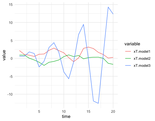 Figure 12.17: Simulated AR(2) models
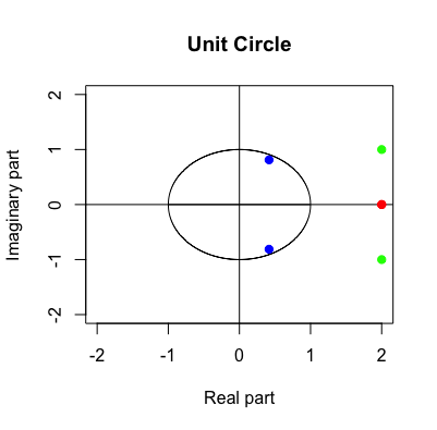 Figure 12.18: Corresponding eigenvalues of AR(2) models
Code of simulated AR(2)
Trade flows
Recall that the directed networks in chapter 10.4 can record the direction of the connections amongst the vertices. Assume that across each edge of this directed network, something flows. This something could be loans (for a network of banks), could be a current (for a network of a circuit), or could be monetary transactions (for a network of international trades). As each network can be denoted by an adjacency matrix \(\mathbf{A}=[a_{ij}]_{n\times n }\), one can let the non-zero entry \(a_{ij}\) in the matrix denote the flows from the vertex \(i\) to \(j\).
The following data table gives a sample of the international trade flows data.
The table is equivalent to a data matrix \(\mathbf{A}\) where \(a_{ij}\) represents the trade flows from country \(i\) (export) to country \(j\) (import).
##         importer
## exporter          ARG          AUS          AUT          BEL          BGR
##      ARG 3.231337e+04 1.078020e+02 2.519563e+01 1.892631e+02 1.703026e+01
##      AUS 3.589711e+01 2.613646e+05 6.584548e+01 4.097345e+02 1.446565e+01
##      AUT 1.006038e+02 7.307719e+02 7.314190e+04 2.189365e+03 5.434811e+02
##      BEL 2.856919e+02 1.260780e+03 3.022729e+03 4.867070e+05 2.946212e+02
##      BGR 9.007073e+00 1.455710e+01 2.828406e+02 9.621429e+02 1.437417e+04
In social phenomena, certain network vertices form more efficient linkages than the others. The structure of such networks often consists of strong ties of interactions between some center vertices and many relatively isolated vertices. This phenomenon is called centrality in network analysis. More specifically, the more a vertex is connected to highly connected vertices, the stronger its centrality. In other words, more connections and more flows seem to endow more power.
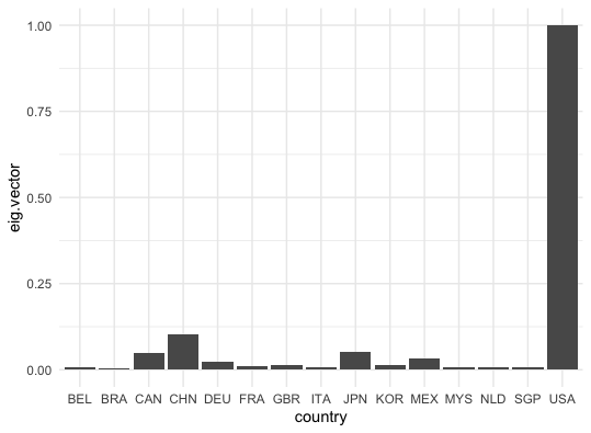 Figure 12.19: Top 15 countries in international trading (2006)
Eigenvalue-eigenvector decomposition of the adjancy matrix can show the centrality in a way that vertices are arranged in a hierarchical relation to specific eigenvector positions. Simiarly to the example of ranking the pages (see chapter 10.4), we can count the total importing trade flows of each country and then rank the countries according to the counting score. Let \(x_{i}\) be the counting score of the country \(i\). We define \(x_i\) as the sum of all the exporting trades multiplying the scores of the corresponding importers: \[x_{i}=\sum_{j}a_{i,j}x_{j},\:\mbox{or say }\mathbf{x}=\mathbf{A}\mathbf{x}.\] It is obvious to see that the score vector \(\mathbf{x}\) is the eigenvector of \(\mathbf{A}\) whose associated eigenvalue is one. In addition, the \(i\)-th entry of the eigenvector represents the \(i\)-th country’s trading strength in this international trade flows data.
Code
Page built: 2021-06-01