11 Matrix Computation

11.1 Gaussian Elimination

Gaussian elimination is a method for solving systems of linear equations by the use of echelon forms. There are many possible ways to solve systems of equations, however, Gaussian elimination is a way that always works. Consider the previous system (10.1) of two unknowns, \(x_1\) and \(x_2\). Its elimination form is given by \[\begin{align*} 0.6x_{1} + 0.3x_{2}=1 & \; & \; &\; & \frac{6}{10}x_{1} + \frac{3}{10}x_{2}=1 \\ & \,& \Rightarrow &\, &\\ -0.3x_{1} + 0.6x_{2} =0 & \; &\; &\; & \frac{15}{20}x_{2}=\frac{1}{2}. \end{align*}\] Before the elimination, \(x_{1}\) and \(x_{2}\) appeared in both equations. After the elimination, the first unknown \(x_{1}\) has disappeared from the second equation. We can solve the elimination form by substituting \(x_{2}=2/3\) back into the first equation.

If we summarize the coefficient as the matrix, the above elimination produces an echelon form of the matrix - an upper triangular matrix.185185 An upper triangular matrix, say \(\mathbf{U}=[u_{ij}]_{n\times n}\), is a matrix satisfying with \([u_{ij}]_{n\times n}=0\) for \(i>j\) and \(u_{ii}\neq0\) for \(i\leq n\). Similarly, the lower triangular matrix, say \(\mathbf{L}=[l_{ij}]_{n\times n }\), satisfies \([l_{ij}]_{n\times n}=0\) for \(i<j\) and \(l_{ii}\neq0\) for \(i\leq n\). With the form, we can solve the system from the bottom upwards. This process of solving the system is called backward substitution. It works for any size of unknowns as long as the system can be eliminated to an upper triangular pattern. The goal of Gaussian elimination is to give an operation to form such a pattern. In above example, we substracted \(x_1\) from the second equation. The step that eliminates \(x_1\) is done by multiplying some factor(s) to the equation(s). In the example, if you mutiple the frist equation by \(0.3/0.6=1/2\), and then substract the first from the second, you will get this triangular form. The multiplier \((0.3)/(0.6)\), consists of two numerics, \(0.3\) and \(0.6\) are the (positive) coefficients of the eliminated unknown \(x_1\) in the second and the first equation, respectively. The coefficient of the eliminated variable is called the pivot.

If we present the eliminated form in terms of matrix, the matrix is \[\left[\begin{array}{cc} \frac{6}{10} & \frac{3}{10}\\ 0 & \frac{15}{20} \end{array}\right].\] Such a staircase matrix format is called the echelon matrix. The nonzero rows of the matrix precede the zero rows. The column numbers of the leading entries, namely the pivots of the nonzero rows, form a staircase type.186186 Note that zero is not a pivot. For the following system, the pivot of \(y\) is zero. \[\begin{align*} 2x+3y =5 & \; & 2x+ 3y =5 &\\ & \, \Rightarrow \, & &\\ 10x+15y =30 & \; & 0y =5. & \end{align*}\] Doing Gaussian elimination on such a system will result in a contradiction. When this happens, it is safe to say that the system has no solution. However, for the system \[\begin{align*} 2x+3y =5 & \; & 2x+ 3y =5 &\\ & \, \Rightarrow \, & &\\ 10x+15y =25 & \; & 0y =0, & \end{align*}\] the second equation \(0y=0\) gives no constraint on \(y\). Then any combination of \(x\) and \(y\) satisfying the first equation will also be the solutions of the second. It means that the system has infinite solutions. Thus, for zero leading entries in the echelon matrix, we may face the situation of either no solution or infinite solutions. In above system, the pivots are \(6/10\) and \(15/20\). To solve \(n\) equations, we need \(n\) pivots.

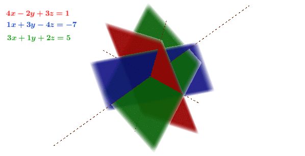Figure 11.1: Gaussian elimination in 3D

Figure 11.1 shows the geometrical interpretation of constructing a reduced echelon form.187187 When the pivots are normalized to one, the echelon form is calle the reduced echelon form. We can see that the procedures (multiplication and substraction) have no effect on the solution point, namely the intersection. Each equation of the system (3D) is represented by a plane (2D). Multiplication extends the plane (which has no visual effect), substraction rotates the plane. None of the operations shift the solution point. This interpretation illuminates some general rules of constructing an echelon form or a Gaussian elimination. The rules can be summarized as follows:188188 These rules can be presented in terms of elimentary matrices, see section[?].

The solutions to a linear system of equations do not change if

1. we swap the order of two rows,

2. multiply a row with a constant ,

3. or add a multiple of another row to a row.

With these rules, let’s consider a general linear system \[\begin{align*} a_{11}x_{1}+\cdots+a_{1n}x_{n} &=y_{1},\\ a_{21}x_{1}+\cdots+a_{2n}x_{n} &=y_{2},\\ \vdots\qquad \quad & \vdots\\ a_{m1}x_{1}+\cdots+a_{mn}x_{n} &=y_{n}. \end{align*}\] If we first work with \(x_{1}\), then two things can happen. Either all \((a_{i1})_{i=1,\dots m}\) are zero, or at least one \(a_{i1}\) of is non-zero. We can do nothing for the first case. For the second case, we reorder the system (rule 1) so that the new \(a_{11}^{'}=a_{i1}\neq0\) is the first pivot. Then we use the mutiplier \(-(a_{21}/a_{11}^{'})\) to subtract \(x_{1}\) from the second equation, use the mutiplier \(-(a_{31}/a_{11}^{'})\) to subtract \(x_{1}\) from the third equation, so on and so forth. These subtractions will eliminate \(x_{1}\) from all equations except the first. The system becomes \[\begin{align*} a_{11}^{'}x_{1}+a_{12}^{'}x_{2}\cdots+a_{1n}^{'}x_{n} &=y_{1}^{'},\\ a_{22}^{'}x_{2}+\cdots+a_{2n}^{'}x_{n} &=y_{2}^{'},\\ \vdots\qquad \quad & \vdots\\ a_{m2}^{'}x_{2}+\cdots+a_{mn}^{'}x_{n} &=y_{n}^{'}, \end{align*}\] where \(a_{ij}^{'}\) are the new coefficients after the swaps and mutiplications. Repeating this procedure, we will confront three possible outcomes when \(m>n\).

The first case is that if at least one equation contains \(0=y_{i}^{*}\neq0\) there is no solution (overdetermined).

In the second case, at the end, there might be equations left of the type \(0=0\). These can just be removed. And we will have an upper triangular form of \(n\) non-zero equation as follows \[\begin{align*} a_{11}^{*}x_{1}+a_{12}^{*}x_{2}+\cdots+a_{1n}^{*}x_{n} &=y_{1}^{*},\\ a_{22}^{*}x_{2}+\cdots+a_{2n}^{*}x_{n} &=y_{2}^{*},\\ \vdots\qquad \quad & \vdots\\ a_{nn}^{*}x_{n} &=y_{n}^{*}, \end{align*}\] where \(a_{ij}^{*}\) and \(y_{i}^{*}\) have new values under the elimination procedure. We can use the backward substitution to solve this system. In this case, there is a unique solution.

In the third case, there are fewer equations than unknowns after the elimination (underdetermined). For example, \[\begin{align*} a_{11}^{*}x_{1}+a_{12}^{*}x_{2}+\cdots+a_{14}^{*}x_{4} &=y_{1}^{*},\\ a_{22}^{*}x_{2}+\cdots+a_{24}^{*}x_{4} &=y_{2}^{*},\\ a_{43}^{*}x_{3}+a_{44}^{*}x_{4} &=y_{3}^{*}. \end{align*}\] We have three equations but four unknonws. In this example, the pivots are for \(x_{1}\), \(x_{2}\) and \(x_{3}\). There is in fact no constraint on the remaining variable \(x_{4}\). Thus, we have an infinite number of solutions.

Among these three cases, the second one is of most interests, because it guarantees a unique solution. The unique solution of this general linear system is a vector called solution vector such that the resulting equations are satisfied for these choices of the variables. When there are multiple solutions, the set of all solutions is called the solution set of the linear system, and two linear systems are said to be equivalent if they have the same solution vector or solution set. The key idea behind the Gaussian elimination is to construct the equivalent systems, i.e. they all have the same solution vector or solution set.

The computation for the unique solution in the second case uses the backward substitution. Given an \(n\times n\) upper triangular matrix \(\mathbf{A}\) with non-zero diagonal entries, and \(\mathbf{b}\in\mathbb{R}^{n}\), the backward substitution is as follows:

1: Criteria: \(\mathbf{A}=[a_{ij}]_{n\times n}, [a_{ij}]_{n\times n}=0\) for \(i>j\) and \(a_{ii}\neq0\) for \(i\leq n\), \(\mathbf{b}\in\mathbb{R}^n\).
2: Variable: \(\mathbf{x}\in\mathbb{R}^n\)
3: FOR \(i\) from \(n\) to \(1\) DO:
4: \(\qquad\) \(x_{i}=(b_{i}-a_{i,i+1}x_{i+1}-\cdots-a_{i,n}x_{n})/a_{i,i}\)
5: END FOR-\(i\) LOOP
6: RETURN \(\mathbf{x}\)

The backward substitution is easy to implement. But when the system grows larger (more unknowns, more equations), a simple algorithm such as backward substitution may become costly. The complexity of backward substitution is given as follows:189189 The current computers store real numbers in a format called floating points, i.e. a real number using a block of \(64\) bits - \(0\)s and \(1\)s. When computers carry out an arithmetic operation such as addition or subtraction on numbers, a very rough estimate of the time required to proceed this computation can be calculated by counting the total number of floating point operations. The complexity of an operation is the (minimum) number of floating point operations required to carry it out. From the bottom upwards in the echelon form, the first step only requires a division of \(a_{nn}\). The next step requires one multiple, one subtraction, and one division \(x_{n-1}=(b_{n-1}-a_{nn}x_{n})/a_{n-1,n-1}\), so three operations. In \(k\)-step, the operations contain \(k-1\) multiplies, \(k-1\) subtractions, and one division, hence \(2k-1\) operations in total. Thus, the total number of operations for backward substitution of an \(n\)-variables, \(n\)-equation echelon system is \(1+3+\cdots+(2n-1)=n^{2}\). But the inner product of two \(n\)-vectors only costs \(2n-1\) operations: \(n\) scalar mutiplications and \(n-1\) scalar additions. We can imagine that for a large \(n\), the complexity of the backward substitution is much larger than that of the inner product.190190 In certain settings it is handy to use the “Big-Oh” notation when an order of magnitude assessment of work suffices. Inner products are \(O(n)\), matrix-vector products are \(O(n^{2})\), and matrix-matrix products are \(O(n^{3})\).

11.2 Matrix Inverses

When there is little prospect in proceeding, one solution is to take a backward step, to re-examine the passing path and hopefully to explore a possible way out. The solution for many difficult problems in mathematics could also be found if the problems were expressed in the inverse manner. In this sense, the matrix inversion could illuminate a deeper mechanism regarding the matrix computation.

We knew that it is straightforward to compute the quantity \(1/a\) if \(a\in\mathbb{R}\). But to compute \(1/\mathbf{A}\) for a matrix \(\mathbf{A}\), we should be sure that the inverse \(1/\mathbf{A}\) makes sense. That is, the laws of matrix multiplication are not violated under the inversion. Notice that the order matters in a matrix multiplication. We do not expect \(\mathbf{A}\mathbf{B}=\mathbf{B}\mathbf{A}\) in general. For inversion, the order implies that there exists two types of pseudo inversions of a matrix. That is, for a matrix \(\mathbf{A}\in\mathbb{R}^{m\times n}\) with \(m,n\in\mathbb{N}\), we expect to have a left inverse and a right inverse of the matrix \(\mathbf{A}\). If a matrix \(\mathbf{B}\in\mathbb{R}^{n\times m}\) satisfies \(\mathbf{B}\mathbf{A}=\mathbf{I}\), then \(\mathbf{B}\) is called a left inverse of \(\mathbf{A}\). The matrix \(\mathbf{A}\) is said to be left invertible if a left inverse exists. Similarly, if \(\mathbf{A}\mathbf{C}=\mathbf{I}\), then \(\mathbf{C}\in\mathbb{R}^{n\times m}\) is called the right inverse of \(\mathbf{A}\). The right inverse \(\mathbf{B}\) and the left inverse \(\mathbf{C}\) can be completely different matrices. If the right inverse \(\mathbf{B}\) and the left inverse \(\mathbf{C}\) are different, then the inverse matrix of \(\mathbf{A}\) does not exist.191191 Usually the left or right inverses are not unique. There may be more than one left or right inverses. When people refer to an invertible matrix, they often implicitly refer to a square matrix (\(n=m\)) whose left inverse and right inverse are equivalent.

For a square matrix \(\mathbf{A}\in\mathbb{R}^{n\times n}\), the matrix \(\mathbf{A}\) is invertible if there exists a matrix \(\mathbf{A}^{-1}\) such that \[\mathbf{A}^{-1}\mathbf{A}=\mathbf{I},\quad\mbox{and }\quad\mathbf{A}\mathbf{A}^{-1}=\mathbf{I}.\]192192 Note that for square matrices, left inverse, right inverse and inverse \(\mathbf{A}^{-1}\) are equivalent. That is, if \(\mathbf{A}\) is right invertible, then it is left invertible, and vice-versa. This inverse is unique. Otherwise, suppose that both \(\mathbf{B}\) and \(\mathbf{C}\) work as inverses to the square matrix \(\mathbf{A}\), we can show that these matrices must be identical. The associative and identity laws of matrices yield \[\mathbf{B}=\mathbf{B}\mathbf{I}\overset{(a)}{=}\mathbf{B}(\mathbf{A}\mathbf{C})\\=(\mathbf{B}\mathbf{A})\mathbf{C}=\mathbf{I}\mathbf{C}=\mathbf{C}.\] If \(\mathbf{A}^{-1}\) exists, then \(\mathbf{A}\) is said to be invertible or nonsingular. Otherwise, we say \(\mathbf{A}\) is singular or non-invertible.

The study of matrix inversion is equivalent to the study of solving a linear equation system. Assume \(\mathbf{A}\in\mathbb{R}^{m\times n}\), \(\mathbf{b}\in\mathbb{R}^{m}\), \(\mathbf{x}\in\mathbb{R}^{n}\), and the linear system \(\mathbf{A}\mathbf{x}=\mathbf{b}\). The solution of the system \(\mathbf{x}=\mathbf{A}^{-1}\mathbf{b}\) includes the matrix inversion \(\mathbf{A}^{-1}\). As for the square matrix \(\mathbf{A}\in\mathbb{R}^{n\times n}\), the inverse \(\mathbf{A}^{-1}\), if it exists, is unique. For example, consider the solution of the following system \[\begin{split}x_{1}= & y_{1}\\ x_{2}= & y_{1}+y_{2}\\ x_{3}= & y_{1}+y_{2}+y_{3} \end{split} \Leftrightarrow\mathbf{x}=\left[\begin{array}{ccc} 1 & 0 & 0\\ 1 & 1 & 0\\ 1 & 1 & 1 \end{array}\right]\left[\begin{array}{c} y_{1}\\ y_{2}\\ y_{3} \end{array}\right]=\mathbf{A}^{-1}\mathbf{y}\] As we will see, \(\mathbf{A}^{-1}\), the lower triangular matrix, is both the left and the right inverse of \(\mathbf{A}\). \[\left[\begin{array}{ccc} 1 & 0 & 0\\ -1 & 1 & 0\\ 0 & -1 & 1 \end{array}\right]\left[\begin{array}{ccc} 1 & 0 & 0\\ 1 & 1 & 0\\ 1 & 1 & 1 \end{array}\right]=\left[\begin{array}{ccc} 1 & 0 & 0\\ 1 & 1 & 0\\ 1 & 1 & 1 \end{array}\right]\left[\begin{array}{ccc} 1 & 0 & 0\\ -1 & 1 & 0\\ 0 & -1 & 1 \end{array}\right]=\left[\begin{array}{ccc} 1 & 0 & 0\\ 0 & 1 & 0\\ 0 & 0 & 1 \end{array}\right].\] namely, \(\mathbf{A}^{-1}\mathbf{A}=\mathbf{A}\mathbf{A}^{-1}=\mathbf{I}\). Thus, we expect to have a unique solution for the system \(\mathbf{A}\mathbf{x}=\mathbf{b}\) when \(\mathbf{A}\) is invertible.193193 For \(\mathbf{A}\in\mathbb{R}^{m\times n}\), when \(m<n\), the number of unknown variables \((x_{i})_{i\leq n}\) is more than the number of equations, the system \(\mathbf{A}\mathbf{x}=\mathbf{b}\) is an overdetermined linear system. When \(n>m\), the system is an underdetermined linear system. Therefore, the computational procedure of solving a linear system is equivalent to finding an inverse.

The equivalence can be revealed by consideroing the Gaussian elimination in the matrix form. Recall that the idea of Gaussian elimination is to reduce the system of equations to an echelon form by certain legitimate and reversible algebraic operations (elementary operations). In the echelon form, we can easily see what the solutions to the system are, if there are any. In matrix computations, these elementary operations are summarized by the so-called elementary matrices. The elementary matrice provide elementary operations, such as row or column permutations that are transferred from the identity matrix \(\mathbf{I}\) by some simple invertible operations. Thus, all elementary matrices are invertible matrices as the elementary operations are invertible. Recall the elementary operations in the Gaussian elimination:

1. The order of two equations can be swapped: Permutations

2. Multiplying an equation by a nonzero constant: Scaling

3. An equation can be replaced by the sum of itself and a nonzero multiple of any other equation: Replacement. In particular, the row can be replaced by the sum of that row and a nonzero multiple of any other row; that is: \(\mbox{row}_{i}=\mbox{row}_{i}-a_{ij}\mbox{row}_{j}\).

These operations can also be stated in an elementary matrix form. For example: \[ \left[\begin{array}{cccc} 1 & 0 & 0 & 0\\ 0 & 1 & 0 & 0\\ -2 & 0 & 1 & 0\\ 0 & 0 & 0 & 1 \end{array}\right]\left[\begin{array}{c} x_{1}\\ x_{2}\\ x_{3}\\ x_{4} \end{array}\right]=\left[\begin{array}{c} x_{1}\\ x_{2}\\ -2x_{1}+x_{3}\\ x_{4} \end{array}\right]. \] It is obvious that the matrix is an elementary matrix, and the matrix does the job as the subtraction and mutiplication steps in the Gaussian elimination. Let \(\mathbf{E}_{ij}(d)\) be the replacement elementary matrix for the elementary operation of adding \(d\) times the \(j\)-th row to the \(i\)-th row. The elementary matrix (operation) \(\mathbf{E}_{ij}(d)\) of switching the \(i\)-th and \(j\)-th rows can always be undone by applying \(\mathbf{E}_{ji}(-d)\) such that \[\mathbf{E}_{ij}(d)\mathbf{E}_{ji}(-d)=\mathbf{E}_{ji}(-d)\mathbf{E}_{ij}(d)=\mathbf{I}.\] We can apply this elementary matrix for constructing the triangular matrix (echelon form).

Similarly, let \(\mathbf{E}_{ij}\) be the permutation elementary matrix of switching the \(i\)-th and \(j\)-th rows of the matrix, and let \(\mathbf{E}_{i}(c)\) be the scaling elementary matrix of multiplying the \(i\)-th row by the non-zero constant \(c\). They are also invertible.194194 The diagonal square matrix is not an elementary matrix. But if \(\mathbf{A}\) is a diagonal square matrix with nonzero diagonal, then it is always invertible. \[\mathbf{A}=\left[\begin{array}{cccc} a_{1} & 0 & \cdots\\ 0 & a_{2} & 0 & \cdots\\ \vdots & & \ddots\\ 0 & \cdots & & a_{n} \end{array}\right],\;\\ \mathbf{A}^{-1}=\left[\begin{array}{cccc} a_{1}^{-1} & 0 & \cdots\\ 0 & a_{2}^{-1} & 0 & \cdots\\ \vdots & & \ddots\\ 0 & \cdots & & a_{n}^{-1} \end{array}\right].\] We denote the diagonal matrix via \(\mathbf{A}=\mbox{diag}(a_{1},\dots,a_{n})\).

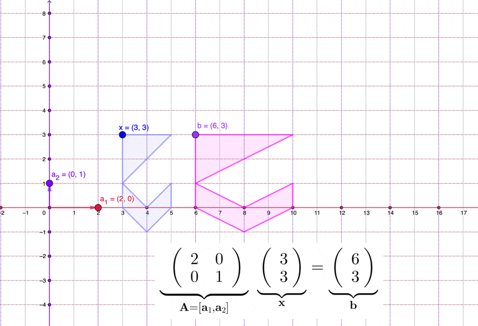Figure 11.2: Matrices transform a set of vectors in two dimensions

For some vectors in \(\mathbb{R}^n\), a matrix in \(\mathbb{R}^{n\times n}\) can transform these vectors into new positions in \(\mathbb{R}^n\). See figure 11.2 for an illustration in \(\mathbb{R}^2\). As \(\mathbf{E}_{ij}(d)\) always satisfies the matrix multiplication laws, for \(\mathbf{A}\mathbf{x}=\mathbf{b}\), multiplying both sides by \(\mathbf{E}_{ij}(d)\) gives a transformed system \(\mathbf{E}_{ij}(d)\mathbf{A}\mathbf{x}=\mathbf{E}_{ij}(d)\mathbf{b}\). The solution(s) \(\mathbf{x}^{*}\) of the original system will still be the solution(s) of the transformed system \(\mathbf{E}_{ij}(d)\mathbf{A}\mathbf{x}^{*}\). Thus \(\mathbf{A}\mathbf{x}=\mathbf{b}\) and \(\mathbf{E}_{ij}(d)\mathbf{A}\mathbf{x}=\mathbf{E}_{ij}(d)\mathbf{b}\) are two equivalent systems.

The following illustration gives the compution of the inverse \(\mathbf{A}^{-1}\) in terms of the elementary matrices. Consider the Gaussian elimination of \[\begin{align*} 2x_{1}-x_{2} =1 & \; & x_{1}+ x_{2} =-5 &\\ & \, \Rightarrow \, & &\\ 4x_{1}+4x_{2} =20 & \; & -3x_{2} =-9. & \end{align*}\] The associated procedure of elementary matrices is given by \[ \mathbf{E}_{21}(-2)\mathbf{E}_{1}(1/4)\mathbf{E}_{12}\left[\begin{array}{cc} 2 & -1\\ 4 & 4 \end{array}\right]\left[\begin{array}{c} x_{1}\\ x_{2} \end{array}\right]= \mathbf{E}_{21}(-2)\mathbf{E}_{1}(1/4)\mathbf{E}_{12}\left[\begin{array}{c} 1\\ 20 \end{array}\right] \\ \Rightarrow\mathbf{E}_{21}(-2)\mathbf{E}_{1}(1/4)\left[\begin{array}{cc} 4 & 4\\ 2 & -1 \end{array}\right]\left[\begin{array}{c} x_{1}\\ x_{2} \end{array}\right]= \mathbf{E}_{21}(-2)\mathbf{E}_{1}(1/4)\left[\begin{array}{c} 20\\ 1 \end{array}\right] \\ \Rightarrow\mathbf{E}_{21}(-2)\left[\begin{array}{cc} 1 & 1\\ 2 & -1 \end{array}\right]\left[\begin{array}{c} x_{1}\\ x_{2} \end{array}\right] =\mathbf{E}_{21}(-2)\left[\begin{array}{c} 5\\ 1 \end{array}\right] \\ \Rightarrow\left[\begin{array}{cc} 1 & 1\\ 0 & -3 \end{array}\right]\left[\begin{array}{c} x_{1}\\ x_{2} \end{array}\right] =\left[\begin{array}{c} 5\\ -9 \end{array}\right]. \] The backward substitution can also be done by the elementary matrices. Continue our previous representation of the triangular matrix. \[ \mathbf{E}_{12}(-1)\mathbf{E}_{2}(-1/3)\left[\begin{array}{cc} 1 & 1\\ 0 & -3 \end{array}\right]\left[\begin{array}{c} x_{1}\\ x_{2} \end{array}\right]= \mathbf{E}_{12}(-1)\mathbf{E}_{2}(-1/3)\left[\begin{array}{c} 5\\ -9 \end{array}\right] \\ \Rightarrow\mathbf{E}_{12}(-1)\left[\begin{array}{cc} 1 & 1\\ 0 & 1 \end{array}\right]\left[\begin{array}{c} x_{1}\\ x_{2} \end{array}\right] =\mathbf{E}_{12}(-1)\left[\begin{array}{c} 5\\ 3 \end{array}\right] \\ \Rightarrow\left[\begin{array}{cc} 1 & 0\\ 0 & 1 \end{array}\right]\left[\begin{array}{c} x_{1}\\ x_{2} \end{array}\right] =\left[\begin{array}{c} 2\\ 3 \end{array}\right]. \] Now, we’ve reached the solution \(\mathbf{x}=\mathbf{A}^{-1}\mathbf{b}\) where \(\mathbf{A}^{-1}=\mathbf{E}_{12}(-1)\mathbf{E}_{2}(-1/3)\mathbf{E}_{21}(-2)\mathbf{E}_{1}(1/4)\mathbf{E}_{12}\). This procedure is feasible for any linear system \(\mathbf{A}\mathbf{x}=\mathbf{b}\) with the square matrix \(\mathbf{A}\).

Matrix inverse properties: If matrices \(\mathbf{A}\) and \(\mathbf{B}\) are invertible, then \(\mathbf{A}^{\top}\), \(\mathbf{A}^{-1}\), \(\mathbf{B}^{-1}\), and \(\mathbf{A}\mathbf{B}\) are also invertible, and

1. \((\mathbf{A}^{-1})^{-1}=\mathbf{A}\).

2. \((\mathbf{A}\mathbf{B})^{-1}=\mathbf{B}^{-1}\mathbf{A}^{-1}\).195195 The inverse of a product \(\mathbf{A}\mathbf{B}\) comes in an reverse order because the order matters in the matrix mutiplication.

3. \((\mathbf{A}^{-1})^{\top}=(\mathbf{A}^{\top})^{-1}\).

Note that unlike the scalar case, it is hard to say much about the invertibility of \(\mathbf{A}+\mathbf{B}\), even if both \(\mathbf{A}\) and \(\mathbf{B}\) are invertible.

In the Gaussian elimination, we saw that having a unique solution, the pivots of the echelon form needs to be non-zero. If the \(i\)-th pivot is zero, it means that either there is not enough information for solving the variable \(x_{i}\), namely underdetermined, or the system has no solution, namely overdetermined. In this case, it also means that the matrix inversion \(\mathbf{A}^{-1}\) does not exist, since the system cannot provide a unique solution. In other words, the inverse \(\mathbf{A}^{-1}\) exists when \(\mathbf{A}\) has a full set of \(n\) pivots.

We can summarize the conditions regarding the invertibility. Let \(\mathbf{A}\) be an \(n\times n\) matrix. The following statements are equivalent.

1. The matrix \(\mathbf{A}\) is invertible or nonsingular.

2. Given any \(n\times1\) vector \(\mathbf{b}\), the linear system \(\mathbf{A}\mathbf{x}=\mathbf{b}\) has a unique solution.

3. The matrix \(\mathbf{A}\) has a full set of \(n\) pivots. (Namely, \(\mbox{det}(\mathbf{A})\neq0\).)196196 See section 12.1 for the definition of the determinant, \(\mbox{det}\).

4. The system of equations \(\mathbf{A}\mathbf{x}=0\) has the unique solution \(\mathbf{x}=0\).197197 We can prove this statement from 2). Suppose 2) is true, then \(\mathbf{A}\mathbf{x}=\mathbf{b}\) has a unique solution, denoted by \(\mathbf{x}^{*}\). Suppose \(\mathbf{A}\mathbf{x}=0\) has a non-trivial solution, say \(\mathbf{x}=\mathbf{q}\) and \(\mathbf{q}\neq0\), then \(\mathbf{A}(\mathbf{x}^{*}+\mathbf{q})=\mathbf{b}\) is also valid. It means that we have obtained another solution \(\mathbf{x}^{*}+\mathbf{q}\), which contradicts with 2). So \(\mathbf{q}=0\) is the unique solution of \(\mathbf{A}\mathbf{x}=0\).

11.3 Example: LU factorization, Forward and Backward Substitution, Distributed Computation

Gaussian elimination is an approach that always works. But in terms of computational efficiency, very often it may not be the case. For example, a linear system \(\mathbf{A}\mathbf{x}=\mathbf{b}\) with as many as \(100,000\) variables of the vector \(\mathbf{x}\) often arise in the solution of differential equations. The coefficient matrix \(\mathbf{A}\) for the system is sparse; that is, a large percentage of the entries of the coefficient matrix are zero. Inverting \(\mathbf{A}\) directly in this situation triggers a high computational cost. Other iterative approaches may provide more efficient solutions if they can utilize some special factors of the matrix \(\mathbf{A}\).

Let’s review the Gaussian elimination procedure. It starts with the last non-zero row, scales all the leading entries on the diagonal to one, then backward substitutes row by row up to the first row. We can think of two phases existing in the Gaussian elimination. The first phase (find and scale the pivots) is forward solving, and the second phase (backward substitution) is backward solving. Many key ideas of computation, when you look at them closely, share such a forward and backward strategy. In matrix computation, this forward and backward procedure can be presented by factorizating one square matrix into two triangular matrices, called the LU decomposition.

The idea behind Gaussian elimination is to convert a given system \(\mathbf{A}\mathbf{x}=\mathbf{b}\) to an equivalent triangular system (echelon form. We have seen that the construction of the upper triangular form is to multiple some elementary matrices. Notice that each replacement matrix \(\mathbf{E}_{ij}(d)\) has a lower triangular structure for \(i<j\).198198 This is the feature of forward solving phase, as the phase eliminates row by row up to the first row. The forward solving phase includes a sequence of multiplicative elementary matrices that can be denoted by a lower triangular matrix \(\mathbf{L}\), e.g. \(\mathbf{L}=\mathbf{E}_{12}^{-1}(d_{1})\mathbf{E}_{23}^{-1}(d_{2})\cdots\). After the forward solving phase, the nonsingular matrix \(\mathbf{A}\) turns into an upper triangular matrix, say \(\mathbf{U}\). These two phases are given as follows:

• LU factorization: Assume a sequence of multiplications to be \(\mathbf{E}_{12}(d_{1})\mathbf{E}_{23}(d_{2})\cdots\mathbf{E}_{ij}(d_{k})\). Triangularizing the system \(\mathbf{A}\mathbf{x}=\mathbf{b}\) is equivalent to \[\mathbf{E}_{12}(d_{1})\mathbf{E}_{23}(d_{2})\cdots\mathbf{E}_{ij}(d_{k})\mathbf{A}\mathbf{x}=\mathbf{E}_{12}(d_{1})\mathbf{E}_{23}(d_{2})\cdots\mathbf{E}_{ij}(d_{k})\mathbf{b},\] or say \(\mathbf{U}\mathbf{x}=\mathbf{c}\) where \(\mathbf{U}\) is \(\mathbf{E}_{12}(d_{1})\mathbf{E}_{23}(d_{2})\cdots\mathbf{E}_{ij}(d_{k})\mathbf{A}\), and \(\mathbf{c}\) is \(\mathbf{E}_{12}(d_{1})\mathbf{E}_{23}(d_{2})\cdots\mathbf{E}_{ij}(d_{k})\mathbf{b}\). Then for the matrix \(\mathbf{U}=\mathbf{E}_{12}(d_{1})\mathbf{E}_{23}(d_{2})\cdots\mathbf{E}_{ij}(d_{k})\mathbf{A}\), we can resolve the matrix \(\mathbf{A}\) by multiplying the product of the inverses \(\mathbf{E}_{ij}^{-1}(d_{k})\cdots\mathbf{E}_{23}^{-1}(d_{2})\mathbf{E}_{12}^{-1}(d_{1})\). Note that any \(\mathbf{E}_{ij}^{-1}(d_{k})\) from the product is also a lower triangular matrix. Thus, the product of the inverses gives a new lower triangular matrix: \(\mathbf{L}=\mathbf{E}_{ij}^{-1}(d_{k})\cdots\mathbf{E}_{23}^{-1}(d_{2})\mathbf{E}_{12}^{-1}(d_{1})\). We have the LU factorization \[\mathbf{A}=\mathbf{E}_{ij}^{-1}(d_{k})\cdots\mathbf{E}_{23}^{-1}(d_{2})\mathbf{E}_{12}^{-1}(d_{1})\mathbf{U}=\mathbf{L}\mathbf{U}.\]

The LU factorization shows that one square system \(\mathbf{A}\mathbf{x}=\mathbf{b}\) is equivalent to two triangular systems \(\mathbf{A}\mathbf{x}=\mathbf{L}(\mathbf{U}\mathbf{x})=\mathbf{L}\mathbf{c}=\mathbf{b}\). In summary, the forward and backward steps solve \(\mathbf{A}\mathbf{x}=\mathbf{b}\) as follows:

1. LU factorization of \(\mathbf{A}\). \(\mathbf{A}=\mathbf{L}\mathbf{U}\).

2. Forward: \(\mathbf{L}\mathbf{c}=\mathbf{b}\)

3. Backward: \(\mathbf{U}\mathbf{x}=\mathbf{c}\)

The factorization can gain a lot computational efficiency. In section 11.1, we saw that the complexity of Gaussian elimination is of the magnitude \(O(n^{3})\), while in the backward substitution step, complexity is of the magnitude \(O(n^{2})\). The decrease of complexity comes with the (upper) triangular structure where the first equation involves all the variables, the second equation involve all but the first, and so forth. In other words, the computational complexity of solving a triangular system is smaller.

The following matrix is a second order difference matrix. It is a discrete counterpart of the second order differentiation, which is used in the diffusion models. Recall that the second difference operation \((x_{i+1}-x_{i})-(x_{i}-x_{i-1})=x_{i-1}-2x_{i}+x_{i+1}\) in chapter 8.5. The matrix form of this operation is given by \[\mathbf{A}\mathbf{x}=\left[\begin{array}{ccccc} 2 & -1 & \cdots & & 0\\ -1 & 2 & -1 & \cdots\\ \vdots & \ddots & \ddots & \ddots & \vdots\\ 0 & \cdots & -1 & 2 & -1\\ 0 & 0 & \cdots & -1 & 1 \end{array}\right]\left[\begin{array}{c} x_{1}\\ x_{2}\\ \vdots\\ x_{n-1}\\ x_{n} \end{array}\right] \\ =-\left[\begin{array}{c} x_{2}-2x_{1}\\ x_{1}-2x_{2}+x_{3}\\ \vdots\\ x_{n-2}-2x_{n-1}+x_{n}\\ x_{n-1}-x_{n} \end{array}\right] =\left[\begin{array}{c} b_{1}\\ b_{2}\\ \vdots\\ b_{n-1}\\ b_{n} \end{array}\right].\] Except the first and the last row, the matrix \(\mathbf{A}\) has the second differences for the rest entries. The system \(\mathbf{A}\mathbf{x}=\mathbf{b}\) numerically approximates the second order differential equation \(\mbox{d}^{2}x(t)/\mbox{d}t^{2}=b(t)\).

The LU factorization of this second difference matrix is \[\left[\begin{array}{ccccc} 2 & -1 & \cdots & & 0\\ -1 & 2 & -1 & \cdots\\ \vdots & \ddots & \ddots & \ddots & \vdots\\ 0 & \cdots & -1 & 2 & -1\\ 0 & 0 & \cdots & -1 & 1 \end{array}\right]=\left[\begin{array}{ccccc} 1 & 0 & \cdots & & 0\\ -1 & 1 & 0 & \cdots\\ \vdots & \ddots & \ddots & \ddots & \vdots\\ 0 & \cdots & -1 & 1 & 0\\ 0 & 0 & \cdots & -1 & 1 \end{array}\right]\left[\begin{array}{ccccc} 1 & -1 & \cdots & & 0\\ 0 & 1 & -1 & \cdots\\ \vdots & 0 & \ddots & \ddots & \vdots\\ 0 & \vdots & 0 & 1 & -1\\ 0 & 0 & \cdots & 0 & 1 \end{array}\right],\] namely \(\mathbf{A}=\mathbf{L}\mathbf{U}\).199199 If one takes a closer look, one may see that the lower traingular matrix \(\mathbf{L}\) is the difference matrix defined in section 10.4, and that \(\mathbf{U}=\mathbf{L}^{\top}\) is the transposed difference matrix. We know that a second order differentiation is about taking the differentiation twice. This is the reason that the second order difference matrix is a product of two first order difference matrices. The transpose operation relates the dual of the inner product rule - integration by parts. We will come back to it in ch[?]. When we solve the differential equation numerically, we discretize a continuous domain on \(t\in [0,T]\) by which we may confront a large set of discrete points, also a large coefficient matrix \(\mathbf{A}\). However, the pattern of \(\mathbf{A}\) is known so that the patterns of LU factorized matrices are known. Instead of computing the Gaussian elimination (\(O(n^{3})\) complexity), we can compute the forward and backward steps \(\mathbf{L}\mathbf{c}=\mathbf{b}\) and \(\mathbf{U}\mathbf{x}=\mathbf{c}\) (\(O(n^{2})\) complexity). This computational gain is significant when \(n\) is large.

The LU factorization is a high-level algebraic description of the Gaussian elimination. The computational efficiency of LU factorization becomes more attractive when the dimension of the matrix grows and the matrix has some structural patterns. The partition of the matrix makes it possible to parallelized the matrix multiplication for otherwise overwhelming system of equations. The idea of effectively parallelization is based on the block-cyclic distribution.

Let’s consider the following matrix \[\mathbf{A}=\left[\begin{array}{cc} \mathbf{A}_{11} & \mathbf{A}_{12}\\ \mathbf{A}_{21} & \mathbf{A}_{22} \end{array}\right].\] Notice that the entries \((\mathbf{A}_{ij})_{i,j\leq2}\) are matrices rather than scalars. The entries \((\mathbf{A}_{ij})_{i,j\leq2}\) are called the block matrices of \(\mathbf{A}\), because they partition \(\mathbf{A}\) into blocks. One virtue of the block form is that the blocks can provide some parallel computations, namely simultaneously evaluating the arithmetic operations. For example, we can partition \(\mathbf{A}\in\mathbb{R}^{n\times n}\) as follows: \[\begin{array}{cc} \left\lceil \begin{array}{cc} \mathbf{A}_{11} & \mathbf{A}_{12}\end{array}\right\rceil & r\\ \left\lfloor \begin{array}{cc} \mathbf{A}_{21} & \mathbf{A}_{22}\end{array}\right\rfloor & n-r\\ \begin{array}{cc} r & n-r\end{array} \end{array}\] where \(\mathbf{A}_{11}\in\mathbb{R}^{r\times r}\) and \(r\) denotes the dimension of this block. The laws of matrix additions and multiplications also hold for the block matrices. The operation regarding the selective blocks are independent of the others.200200 Consider the matrix mutiplication \[\left[\begin{array}{cccc} 1 & 2 & 0 & 0\\ 3 & 4 & 0 & 0\\ 0 & 0 & 1 & 0 \end{array}\right]\left[\begin{array}{cccc} 0 & 0 & 2 & 1\\ 0 & 0 & 1 & 1\\ 0 & 0 & 1 & 0\\ 0 & 0 & 0 & 1 \end{array}\right].\] It can be written as \[\left[\begin{array}{cc} \mathbf{A} & 0\\ 0 & \mathbf{B} \end{array}\right]\left[\begin{array}{cc} 0 & \mathbf{C}\\ 0 & \mathbf{I} \end{array}\right]=\\ \left[\begin{array}{cc} \mathbf{A}\times0+0\times0 & \mathbf{A}\mathbf{C}+0\times\mathbf{I}\\ 0\times0+\mathbf{B}\times0 & 0\times\mathbf{C}+\mathbf{B}\mathbf{I} \end{array}\right]=\\ \left[\begin{array}{cccc} 0 & 0 & 0 & 3\\ 0 & 0 & 2 & 7\\ 0 & 0 & 1 & 0 \end{array}\right]\] where \(\mathbf{A}=\left[\begin{array}{cc} 1 & 2\\ 3 & 4 \end{array}\right]\), \(\mathbf{B}=[1,0] , \mathbf{C}=\left[\begin{array}{cc} 2 & 1\\ -1 & 1 \end{array}\right]\), \(\mathbf{I}=\left[\begin{array}{cc} 1 & 0\\ 0 & 1 \end{array}\right]\). The matrix multiplication \(\mathbf{A}\mathbf{C}\) is only valid when the column dimension of \(\mathbf{A}\) matches the row dimension of \(\mathbf{C}\). Then the matrix computation regarding the blocks can be carried out parallelly in a distributed-memory system, in which the information is collectively stored in the local blocks, and in which the blocks are connected to form a global matrix. When the size of problem grows, the number of blocks also grows but the existing blocks do not. Then the parallelized algorithm simplifies the process of implementing a growing computational problem as such an algorithm can scale. That is, the algorithm remains effective as problem size grows and the number of involved processors increases.

For example, it is possible to have a LU factorization for the block matrix \(\mathbf{A}\): \[\mathbf{A}=\left[\begin{array}{cc} \mathbf{L}_{11} & 0\\ \mathbf{L}_{21} & \mathbf{L}_{22} \end{array}\right]\left[\begin{array}{cc} \mathbf{U}_{11} & \mathbf{U}_{12}\\ 0 & \mathbf{U}_{22} \end{array}\right]\] where \(\mathbf{L}_{ij}\) is the lower triangular matrix, and \(\mathbf{U}_{ij}\) is the upper triangular matrix for \(0<i,j\leq 2\).201201 The algorithm of computing block LU factorization is a bit different from the standard LU. However, the structure of eliminating the block matrix is similar to the use of the replacement elementary matrix such that \[\left[\begin{array}{cc} \mathbf{I} & 0\\ -\mathbf{C}\mathbf{A}^{-1} & \mathbf{I} \end{array}\right]\left[\begin{array}{cc} \mathbf{A} & \mathbf{B}\\ \mathbf{C} & \mathbf{D} \end{array}\right]=\\ \left[\begin{array}{cc} \mathbf{A} & \mathbf{B}\\ \mathbf{0} & \mathbf{D}-\mathbf{C}\mathbf{A}^{-1}\mathbf{B} \end{array}\right].\] The term \(\mathbf{D}-\mathbf{C}\mathbf{A}^{-1}\mathbf{B}\) is called the Schur complement.

11.4 Miscellaneous: Vector Spaces, Operator, Basis

Vector Spaces

So far, the vectors of our concern are from finite dimensions. The finiteness ensures that these vectors can be visualized (on a low dimensional plane) and can be implemented in the computer as concrete objects. A natural question would be, do the rules (axioms) of vectors still hold if we increase the dimension of the vectors to infinity. For infinity, we need to abstract the idea of vectors. The (further) abstraction can enlarge our concerns of the vectors to entirely different kinds of objects. For many of those objects, the study of the abstract ideas is its own reward.

We begin with exploring an abstract concept called the vector space. It could be a practical tool that enables us to understand phenomena that would otherwise escape our comprehension. Recall that the axioms of vectors are regarding the operations of the addition “\(+\)” and scalar multiplication “\(\times\)”. Up till now, we implicitly assume that these operations are taken on \(\mathbb{R}^{n}\). If we need to work on some other context, we need to extend the concept beyond \(\mathbb{R}^{n}\). Notice that the basic entry of a vector is the scalar. For a scalar, it has to satisfy the properties of both operations “\(+\)” and “\(\times\).”202202 That is, both the addition “\(+\)” and scalar multiplication “\(\times\)” over the scalars satisfy commutative and asociative, have identities and satisfy distributive laws. There exist additive inverses for all scalars and multiplicative inverses for all nonzero scalars. An arbitrary collection of numbers within which the four baisc arithmetic operations, namely adition, subtraction, multiplication, and division by a non-zero number, are valid is called a field. A vector space is a set of vectors that consist of scalars from a field.

• Field and vector space: A field \(\mathbb{F}\) is any set where addition “\(+\)” and scalar multiplication “\(\times\)” are well-defined, namely satisfying the arithmetic axioms in section 10.1. The vector space is a non-empty set \(\mathcal{V}\) of vectors whose scalars are fined over a field \(\mathbb{F}\).

Our purpose of generalizing (abstracting) the concept of vectors is first to select the field of scalars.
As we haven seen that the set of real numbers, \(\mathbb{R}\), is a field \(\mathbb{F}=\mathbb{R}\). One can check that the set of rational numbers, \(\mathbb{Q}\), is also a field (\(\mathbb{F}=\mathbb{Q}\)). But neither the set of integers numbers (\(\mathbb{Z}\)) nor that of natural numbers (\(\mathbb{N}\)) is a field.203203 We can easily check this argument by looking at whether a set satisfies the properties of the arithmetic axioms. For \(\mathbb{Q}\), the additive identity is \(0\), the additive inverse is \(-a\) for any \(a\in\mathbb{Q}\), the multiplicative identity is \(1\), and the multiplicative inverse is \(a^{-1}\) for any non-zero \(a\in\mathbb{Q}\). While for \(\mathbb{N}\) and \(\mathbb{Z}\), there is no additive inverse, nor the multiplicative inverse. Although there are many fields are available, for most of our interests, the fields of scalars are chosen to be either real field, \(\mathbb{F}=\mathbb{R}\), or complex field, \(\mathbb{F}=\mathbb{C}\).204204 However, for implementation, the current computers can only process the operations over the rational field \(\mathbb{F}=\mathbb{Q}\). One has to rely on the idea of approximation (see chapter 6.1) to implement the operations on the real and complex fields.

One of the virtues of abstraction is that it allows us to cover many cases with one statement. There are many simple facts that are deducible from the vector space alone. With the standard vector spaces, these facts seem transparently clear. For example, two matrices of the same size follow the arithmatic axioms of addition and scalar multiplication. Thus, matrices are in the vector space. We have seen that a linear function can be represented by an inner product of vectors in chapter 10.2. Now, we can extend our concern to other functions. Let the set of all continuous real-valued functions defined on the domain \([a,b]\) be \(\mathcal{C}[a,b]\). For \(f,g:\mathbb{R}\rightarrow\mathbb{R}\), \(x\in[a,b]\), if \(f,g\) are continous, then we have \(f(x),g(x)\in\mathcal{C}[a,b]\). Because the sum of any two continuous functions is still continuous, and because any constant times a continuous function is also continuous, namely \[(f+g)(x)=f(x)+g(x)\in\mathcal{C}[a,b],\;(cf)(x)=cf(x)\in\mathcal{C}[a,b],\] we conclude that the set \(\mathcal{C}[a,b]\) is a vector space.205205 One can also verify that the operations \(+\) and \(\times\) defined by the arithmetic axioms are valid. Commutative: \((f+g)=(g+f)\), associative: \((f+g)+h=f+(g+h)\). The “zero” (identity for addition) in \(\mathcal{C}[a,b]\) is the constant function \(f(x)=c\) for all \(x\in[a,b]\) with \(c=0\). So we have \(f(x)+0=f(x)\). The negative inverse of \(f(x)\) is \(-f(x)\) . For any \(a,b\in\mathbb{R}\), the distributive law satisfies: \(a(f+g)=af+ag\), \((a+b)g=ag+bg\). The identity for multiplication is the constant function with value one: \(1f(x)=f(x)\). The scalar associative law satisfies: \((ab)f(x)=a(bf(x))\). Thus, we can formally treat the continuous functions on any bounded interval as “vectors.” This is indeed how we store the information of a continuous function in terms of arrays (vectors) of inputs and outputs.

Subspace

From the previous example, one may induce that the set of finite order polynomials belongs to a vector space as these polynomials can be vectorized. On the other hand, we know that polynomials are continuous (see chapter 7), so the set of all polynomials on \([a,b]\) is a subset of \(\mathcal{C}[a,b]\). Thus, we may expect that all polynomials can form a space (a set with some arithmetic laws) that is analogous to the vector space \(\mathcal{C}[a,b]\).

It frequently happens that a certain vector space of interest is a subset of a larger, and possibly better understood, vector space, and that the arithmetic operations are the same for both sets. For example, all polynomial functions are continuous functions. As all continuous functions on a bounded domain can be represented as vectors, so can the polynomial functions. Moreover, as polynomial functions have their own structures, they form a special subspace of the vector space \(\mathcal{C}[a,b]\).

• Subspace: A subspace \(\mathcal{S}\) of a vector space \(\mathcal{V}\) is a set of vectors that contains the zero element of \(\mathcal{V}\), and it is closed under addition and scalar multiplication, namely for \(\mathbf{v}\), \(\mathbf{w}\in\mathcal{S}\), \(\mathbf{v}+\mathbf{w}\in\mathcal{S}\) and \(c\mathbf{v}\in\mathcal{S}\) for any scalar \(c\).207207 Every subspace of a vector space is a subset. But one notable difference between the subspace and subset is that every subspace contains the zero vector.

Let \(\mathcal{P}[0,1]\) denotes all the polynomial functions on interval \([a,b]\), and let \(\mathcal{P}_{n}[a,b]\) is the set of all the \(n\)-th order polynomial functions on \([a,b]\) Consider \(f(x)=a_{1}+a_{2}x+a_{3}x^{2}\) and \(g(x)=b_{1}+b_{2}x+b_{3}x^{2}\) on \([0,1]\). Then \(f,g\in\mathcal{P}_{2}[0,1]\). For any scalar \(c\in\mathbb{R}\), there is \[(f+g)(x)=f(x)+g(x)=(a_{1}+b_{1})+(a_{2}+b_{2})x+(a_{3}+b_{3})x^{2}\in\mathcal{P}_{2}[0,1]\] and \[cf(x)=c(a_{1}+a_{2}x+a_{3}x^{2})\in\mathcal{P}_{2}[0,1],\: cg(x)\in\mathcal{P}_{2}[0,1].\] Hence \(\mathcal{P}_{2}[0,1]\) is closed under the operations of function addition and scalar multiplication. Furthermore, the zero element in \(\mathcal{P}_2[0,1]\) is the constant function \(f(x)=0\) for \(x\in[0,1]\). So all of the arithmetic axioms for a vector space are satisfied. We conclude that all the second order polynomials construct a subspace of the vector space (of all continuous functions).

Usually, we call \(\mathbb{R}^{n}\) a standard real vector space. When we want to measure the similarilty or dissimilarity of two members in a vector space, we need to attach a distance to the space. But to measure the size of an object in the vector space, we just need a norm. For a vector space \(\mathcal{V}\), the norm is a function \(\|\cdot \|:\mathcal{V}\rightarrow [0,\infty)\). When we attach the \(\ell_2\)-norm or Euclidean norm to \(\mathbb{R}^{n}\), then the real vector space becomes the Euclidean vector space. The space \(\mathbb{R}^{n-1}\) is a subspace of \(\mathbb{R}^{n}\).208208 Note that \(\mathbb{R}^{n}\) is a subset of \(\mathbb{C}^{n}\) but \(\mathbb{R}^{n}\) is definitely not a subspace of \(\mathbb{C}^{n}\) as the subset in \(\mathbb{R}^{n}\) is not closed under multiplication by complex scalars. Recall that the Euclidean norm in \(\mathbb{R}^n\) also comes with the inner product. Their relation in the Euclidean vector space \(\mathcal{V}\) can be summarized by \[\|\mathbf{x}\|= \sqrt{\left\langle \mathbf{x},\mathbf{x}\right\rangle }, \, \mathbf{x}\in \mathbb{R}^n.\] However, some norms in the vector spaces cannot induce the inner products.209209 An inner product naturally induces an associated norm but a norm might not have an associated inner product. Recall that an inner product contains the projective property such as the geometrical notions of the length of a vector and the angle between two vectors, and can imply the generalized Pythagoras’ theorem, while a norm or a distance does not necessarily have the projective property. For example, the Pythagoras’ \(\|x+y\|_p = \|x\|_p + \|y\|_p\) does not hold in general for the \(\ell_p\)-norm (\(p\neq 2\)). We will consider some other inner products in ch[?].

So far we mostly consider the examples with \(n\times n\) square matrices. For a general matrix \(\mathbf{A}\in\mathbb{R}^{n\times m}\), we can also think \(\mathbf{A}\in \mathbb{R}^{nm}\). Taking the columns of \(\mathbf{A}\), and taking all the linear combinations of the columns will give a subspace of \(\mathbb{R}^{m}\). As each column has \(m\) entries, so the subspace belongs to \(\mathbb{R}^{m}\).

For \(\mathbf{A}\in\mathbb{R}^{n\times m}\), we will use the rank to denote the number of pivots, and it is written as \(\mbox{rank}A\). If the matrix has \(\mbox{rank}\mathbf{A} =\min(n, m)\), it is said to be a full rank matrix.

Operators

For a vector \(\mathbf{y}\in\mathbb{R}^n\), it is in an \(n\)-dimensional vector space. But for a function \(f \in \mathcal{C}[a,b]\), it is actually in an infinite dimensional vector space (although we can vectorize it into \(n\) finite points \(\mathbf{y}=[y_1,\dots, y_n]\) with \(y_k=f(x_k)\)). So linear function can be thought of a generalization of finite vector. Matrices are about transformation, transfering one vector into another vector. A generalized concept of matrices is called the operator.

• Operator and linear operator: A function that maps elements from one vector space \(\mathcal{V}\) into another vector space \(\mathcal{W}\), say \(\mathbf{T}:\mathcal{V}\rightarrow\mathcal{W}\), is called an operator. A linear function that maps elements from one vector space \(\mathcal{V}\) into another vector space \(\mathcal{W}\) over the same field \(\mathbb{F}\) of scalars, say \(\mathbf{T}:\mathcal{V}\rightarrow\mathcal{W}\) and \[\mathbf{T}(c_{1}\mathbf{u}+c_{2}\mathbf{v})=c_{1}\mathbf{T}(\mathbf{u})+c_{2}\mathbf{T}(\mathbf{v})\] for all \(\mathbf{u},\mathbf{v}\in\mathcal{V}\) and \(c_{1},c_{2}\in\mathbb{F}\), then \(\mathbf{T}\) is a linear operator. In particular, a linear operator becomes a linear functional, if the image of the operator is the field of scalars of the vector space, namely \[\mathbf{T}:\mathcal{V}\rightarrow\mathbb{F}\] where \(\mathbb{F}\) is the field of scalars of \(\mathcal{V}\).

For example, the matrix \(\mathbf{A}\in\mathbb{F}^{m\times n}\) with \(\mathbb{F}=\mathbb{C}\) or \(\mathbb{F}=\mathbb{R}\) is the linear operator \(\mathbf{T}_{\mathbf{A}}:\mathbb{F}^{n}\rightarrow\mathbb{F}^{m}\). It can be expressed as \(\mathbf{T}_{\mathbf{A}}(\mathbf{x})=\mathbf{A}\mathbf{x}\) for \(\mathbf{x}\in\mathbb{F}^{n}\) is a linear operator.210210 An operator \(\mathbf{T}:\mathcal{V}\rightarrow\mathcal{W}\) is said to be invertible if there is an operator \(\mathbf{T}^{-1}:\mathcal{W}\rightarrow\mathcal{V}\) such that the composition \(\mathbf{T}(\mathbf{T}^{-1}(\mathbf{w}))=\mathbf{w}\) and \(\mathbf{T}^{-1}(\mathbf{T}(\mathbf{v}))=\mathbf{v}\) hold for all \(\mathbf{w}\in\mathcal{W}\) and \(\mathbf{v}\in\mathcal{V}\). For an \(n\times n\) matrix \(\mathbf{A}\), the linear operator \(\mathbf{T}_{\mathbf{A}}(\mathbf{x})=\mathbf{A}\mathbf{x}\) is invertible if and only if \(\mathbf{A}\) is an invertible matrix. For an invertible linear operator \(\mathbf{T}:\mathcal{V}\rightarrow\mathcal{W}\), we say the two vector spaces \(\mathcal{V}\) and \(\mathcal{W}\) are isomorphic, and the mapping \(\mathbf{T}\) itself is called an isomorphism. For matrices, \(\mathbb{R}^{m\times n}\) is isomorphic to \(\mathbb{R}^{mn}\).

For the purpose of generalization, we often designate linear functions by linear operators. For example, all the differentiable functions can be associated with an operator defined by \(\mathbf{T}(f(x))=\frac{\mbox{d}f}{\mbox{d}x}\). We can see that the operator obeys the linear rule such that \[\begin{align*}\mathbf{T}(c_{1}f(x)+c_{2}g(x)) &=\frac{\mbox{d}}{\mbox{d}x}(c_{1}f(x)+c_{2}g(x))\\ =c_{1}\frac{\mbox{d}f}{\mbox{d}x}+c_{2}\frac{\mbox{d}g}{\mbox{d}x}&=c_{1}\mathbf{T}(f(x))+c_{2}\mathbf{T}(g(x)). \end{align*}\] Therefore, differentiation is a linear operator on the space of all differentiable functions. Similarly,we can consider this operator is the abstract analogue of the finite difference matrix.

Basis

The set of all linear combinations of finitely many members \(\{\mathbf{v}_{i}\}_{i=1}^{n}\) of a vector space \(\mathcal{V}\) is called the span of \(\mathcal{V}\), denoted by \(\mbox{span}(\mathcal{V})\) or \(\mbox{span}\{\mathbf{v}_{1},\dots,\mathbf{v}_{n}\}\) such that \[\mbox{span}(\mathcal{V}):=\left\{ \sum_{i=1}^{n}c_{i}\mathbf{v}_{i}\,|n\in\mathbb{N},c_{i}\in\mathbb{F},\mathbf{v}_{i}\in\mathcal{V}\mbox{ for any }i\right\}\] where \(\mathbb{F}=\mathbb{C}\) or \(\mathbb{F}=\mathbb{R}\). If \(\mathcal{V}=\mbox{span}\{\mathbf{v}_{1},\dots,\mathbf{v}_{n}\}\), we say that \(\{\mathbf{v}_{1},\dots,\mathbf{v}_{n}\}\) is a spanning set for the vector space \(\mathcal{V}\).

A vector \(\mathbf{v}_{i}\) is redundant if the span \(\mbox{span}\{\mathbf{v}_{1},\dots,\mathbf{v}_{n}\}\) does not change when \(\mathbf{v}_{i}\) is removed. In data science, the spanning set that involves the ordered elements (vectors) is called a data list.

Since \(\mbox{span}(\mathcal{V})\) is the vector space that consists of all finite linear combinations of the vectors in \(\mathcal{V}\), all information/regulations about this space is contained in \(\mathcal{V}\). Thus if we wish to think of a vector space as a span of a certain set, then it makes sense to choose that set as small as possible, namely without any redundant vector. This leads to the notion of a basis.

Consider a set of vectors, \(\mathbf{x}_{1},\mathbf{x}_{2},\dots,\mathbf{x}_{n}\). They are said to be linearly independent, if the equation\[a_{1}\mathbf{x}_{1}+a_{2}\mathbf{x}_{2}+\cdots+a_{n}\mathbf{x}_{n}=0\] has only one solution \(a_{1}=a_{2}=\cdots=a_{n}=0\). If there is at least one other solution, then the set of vectors is linearly dependent.211211 One of these vectors can be written as a linear combination of the others if and only if they are linearly dependent.

• Basis: A basis for the vector space \(\mathcal{V}\) is a spanning set of vectors \(\mathbf{v}_{1},\dots,\mathbf{v}_{n}\) that are linearly independent.

In other words, a basis is a minimal spanning set. This would allow us to economically “represent” the vector space that we are interested in, thereby letting us view the basis as some sort of “nucleus” of the space that it spans.212212 To see this, if \(\mathcal{V}=\mbox{span}\{\mathbf{\mathbf{v}}_{1},\dots,\mathbf{v}_{n}\}\), and if the set \(\{\mathbf{v}_{1},\dots,\mathbf{v}_{n}\}\) has a redundant vector, we can obtain a smaller spanning set of \(\mathcal{V}\) by deleting the redundant vector. Continue this procedure until no more redundant vector left in the spanning set, then we get the basis of \(\mathcal{V}\).

One idea that is strongly embedded in much economics is about representing the preferences - to find a basis of possibile preferences for constructing the utility function. Imagine yourself in the toilet paper aisle at the supermarket. Are you really going to review all brands on offer, comparing them for price, softness, or absorption and then making of these factors a “utility” function for maximization? Highly unlikely. What most people will do is have some idea of what is “good enough” and then pick up one of those “good enough” options. The basis describes a set of decision-making strategies that are good enough to be treated as options in our choice set. The utility representation theorem(s) is to make sure that those acceptable options can be quantified.213213 Technically speaking, the theorem says that there exists a utility function that can quantify all the preferences and preserve the partial order of preferences in the mapping.

I breifly list the logic of the theorem(s). The representation results are deduced by the fact that every vector space has a basis.214214 The proof of this statement is based on axiom of choice… Suppose that any preference of our choice set \(\mathcal{X}\) (a partially ordered set) can be stated as an element in a vector space, then \(\mathcal{X}\) should belong to a vector space. In fact, a utility function is a norm mapping from such a vector space to the real number field. Since every vector space has a basis, the utility function defined on such a basis can represent all the possible (vectorized) preferences.215215 The (partial) order can be preserved as long as the function has some sorts of continuous properties (real-valued convex functions - namely norms - defined on convex sets in a vector space) which will be given in ch[?].